Different degrees of price elasticity of supply describes the different nature of the product and their volume of supply as a reflection of the change in price. For example, the zero price elasticity of supply indicates that the volume of supply will not change with change in price. This means elasticity of supply is zero when there is a fixed supply of the commodity. Therefore, calculation or measurement of price elasticity of supply is needed to understand the nature of the product and its relation with change in prices. Economists have developed different three methods of measurement of price elasticity of supply. They are as below;

The short explanation of all three methods of measurement of price elasticity of supply is presented below.

Percentage/Proportion Method

Under the percentage/proportionate method of measurement of price elasticity of supply, the percentage change in quantity supply is to be divided by the percentage change in the price of the commodity to measure the coefficient of price elasticity of supply. The following formula has been to measure supply elasticity according to the percentage method.

E_S=Percentage or Proportionate change in quantity supply/ Percentage or Proportionate change in the price of the product

Or E_S=%ΔQ/%ΔP or, E_S= (ΔQ/Q)*100/ (ΔP/P)*100 = (ΔQ/ΔP)* (P/Q)

Where ΔQ=Q₂-Q₁; ΔP=P₂-P₁; P₁=Initial price; P₂=New price; Q₁=Initial supply quantity; Q₂= New supply quantity; ΔQ=Change in supply quantity; ΔP=Change in the price of the commodity; and E_S= Coefficient of measurement of price elasticity of supply

For Example, if the price falls from Rs. 150 to Rs. 120 and as a result, the quantity supply decreases from 100 units to 90 units. In this case, calculate the price elasticity of supply by percentage or proportionate method. 

Here,

Initial Price (P₁) = Rs. 150; new price (P₂) = 120, so ΔP=-30

Initial Supply (Q₁) =100 units; new quantity (Q₂) = 90 units, so ΔQ= -10 units.

So, E_S=%ΔQ/%ΔP= (-10/100)*100/ (-30/150)*100= 10%/20%=0.5

Here the coefficient of price elasticity of supply is o.5. It indicates that a 1% decrease in price leads to a decrease in 0.5 % in supply quantity.

Point/Geometric Method

If the price elasticity of supply is to calculate at a finite point on a supply curve then point method is suitable to use. This method is related to the measurement of responsiveness of quantity supply to change in the price of the product if they are changed by a small amount. The value or coefficient of price elasticity of supply differs along a linear and curve-linear supply curve.  The following section presents the measurement of price elasticity of supply under point method in different cases.

Linear Supply Curve

The following formula is used to measure the price elasticity of supply at any particular point on a supply curve.

E_S=%ΔQ_S/%ΔP or, E_S= (ΔQ_S/ ΔP)*(P/Q_S)

The figure given below helps us to measure the price elasticity of the supply by point method in the case of the linear supply function.

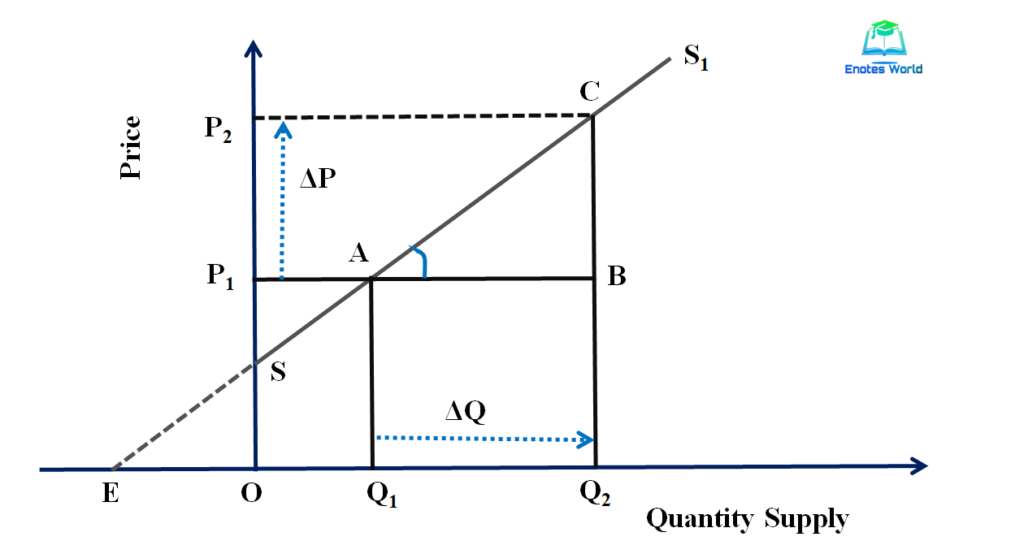
In the above figure, SS₁ is the linear supply curve showing a positive relationship between price and supply of goods. Suppose we want to compute elasticity of supply at a point A on the linear supply curve.  At point A, the initial price is P₁ and the initial supply Q₁. Suppose there is an increase in price from P₁ to P₂ that causes an increase in quantity supply from Q₁ to Q₂. Now from price P₁ let us draw a perpendicular P₁B to meet CQ₂ at point B. The supply curve is extended to meet the x-axis at point E.

Now from the figure, we can see that; ΔQ_S=Q₁Q₂ ΔP= P₁P₂

Thus,

E_S= (ΔQ_S/ ΔP)*(P/Q_S) ———- (i)

Or,    E_S= (Q₁Q₂/ P₁P₂)*(OP₁/OQ₁)

Or,    E_S= (AB/BC)*(AQ₁/OQ₁) ——– (ii)

Now in ΔABC and ΔAEQ₁

<BAC=<AEQ₁ (Corresponding angles)

<ABC=<AQ₁E (Right angles)

<ACB=<EAQ₁ (Remaining angles)

Thus, ΔABC and ΔAEQ₁ are similar. The property of similar triangles is that their corresponding sides are proportional.

So,

AB/EQ₁=BC/Q₁A

Or     AB/BC= EQ₁/ Q₁A——- (iii)

Now substituting the value of equation (iii) into the equation (ii) we get,

E_S= (EQ₁/Q₁A)*(AQ₁/OQ₁)

Or,    E_S= EQ₁/OQ₁———– (iv)

Thus, under the point method of measurement of price elasticity of supply, the elasticity can be measured by using the formula quoted in equation (iv).

Case-I: When Supply Curve has Positive Y-Intercept

The following figure shows the case of a linear supply curve with a positive y-intercept or positive Y-axis.

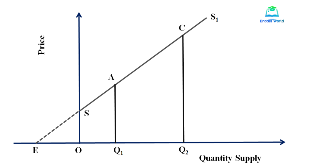
In the above figure, the supply curve is SS₁ and its extension has cur Y-axis and touches X-axis at point E left to the origin. The point price elasticity of supply at point A can be measured as;

Point price elasticity of supply at point A= EQ₁/OQ₁>1

Therefore if the linear supply curve intersects Y-axis or if it has a positive Y-intercept or if the linear supply curve touches X-axis at a point left to the origin then point price elasticity of supply is relatively elastic or greater than one.

Case-II: When the Supply Curve Cuts the Quantity axis and has a Negative Y-Intercept

The following figure shows the case of a liner supply curve with a negative Y-intercept.

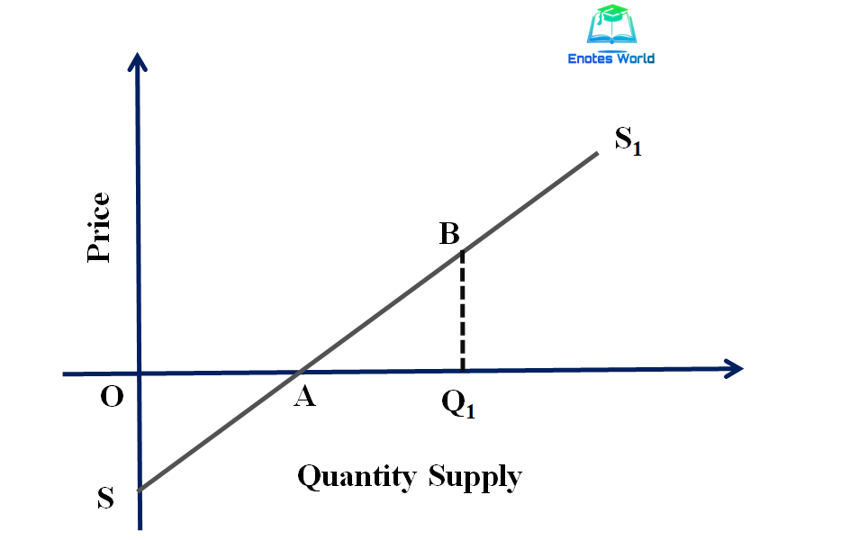
In the figure, the linear supply curve SS₁ has cut the X-axis at a point right to the origin but made a negative Y-intercept. The point price elasticity at point B on the supply curve is measured as;

Point price elasticity of supply at point B= AQ₁/OQ₁<1

Thus, if the supply curve intersects X-axis or made negative Y-intercept, then the elasticity of supply is relatively inelastic or the price elasticity of supply is less than one.

Case-III: When Linear Supply Curve Passes Through the Origin

In the case of the linear supply, curve passes through the origin then the elasticity of supply is unitary elastic or equal to one. The following figure shows the case of a linear supply curve passing through the origin.

In the above figure, the linear supply OS curve passes through the origin. The point price elasticity in case of linear supply curve passing through origin is equal to one. So,

Point price elasticity of supply at point B= OQ₁/OQ₁=1

Non-Linear Supply Curve

The supply curve is not always a straight line and sometimes it may be non-linear. The measurement of price elasticity of supply in the case of a non-linear supply curve can be shown with the help of the following diagram.

In the above figure, SS₁ is the non-linear supply curve. In the case of the non-linear supply curve, to measure point price elasticity or to measure price elasticity of supply at any particular point we have to draw a straight line that is tangent to that particular point where we have to calculate elasticity and then we have to apply the same producer of measurement of price elasticity of supply like linear supply curve case.

Suppose we have to compute the point price elasticity of supply at point A on the given non-linear supply. The tangent line T₁ has drawn passing through point A which intersects the price axis at point P1 and meets horizontal axis at point M. Similarly, tangent lines T₂ and T₃ have also drawn passing through points B and C respectively. Thus the elasticity at these points can be measured as;

Therefore, if the tangent straight line to the supply curve passes through Y-axis or meets X-axis at a point lest to the origin then elasticity of supply is greater than one. Similarly, if the tangent line passes through origin elasticity of supply is unitary elastic and if the tangent line passes through X-axis then the price elasticity of supply is less than one.

Arc/Mid-Point/Average Method

When there is a relatively larger change in price and quantity supply then the arc method is suitable to measure the price elasticity of supply. This method measures the price elasticity of supply by taking the average value or mid-value of both rice and supply quantity. The following formula is used to measure supply elasticity under the arc method.

Where ΔQ_S=Change in supply quantity=Q_S2-Q_S1; ΔP=Change in price=P₂-P₁; P₁=Initial price; P₂= New price; Q_S1=Initial supply; Q_S2=New supply quantity; and E_S= Coefficient of measurement of price elasticity of supply

References and Suggested Readings

Kanel, N.R. and et. al. (2016). Business Economics. Kathmandu: Buddha Publications

Mankiw, N.G. (2009). Principles of Microeconomics. New Delhi: Centage Learning India Private Limited

Salvatore, Dominick. (2003). Microeconomics: Theory and Application. Oxford University Press, Inc.