Contents
Concept of Indifference Curve (IC)
In the microeconomic analysis, an indifference curve (IC) is a graph that shows different combinations of two goods or services that provides the same level of total satisfaction to the consumers. A consumer is always indifferent among any of the bundles of two goods on an indifference curve as they all provide the same satisfaction; the consumer has no preference for one combination over the other. Here we will discuss the assumptions and properties of the indifference curve.
Indifference curves are supposed to be very important tools while analyzing utility as they are used to represent an ordinal measure of the tastes and preferences of the consumer and to display in what way the buyer optimizes pleasure or satisfaction from his or her outlay income.
An English Economist, Francis Ysidro Edgeworth, invented the technique of indifference curve nearly at the end of the 19th century. In the 1880’s he employed it to show the possibility of exchange between two persons but he did not employ different types of curves to explain consumer demand. The Italian economist Vilfredo Pareto polished and applied the concept more expansively than before in the early nineties. Finally, in the 1930’s it was greatly extended by two English economists R.G.D Allen and J.R Hicks.
Meaning and Definitions of Indifference Curve
An indifference curve (IC) is the locus of all those combinations of any two goods that yields the same level of satisfaction to the consumer. It represents the same level of satisfaction of a consumer from different bundles of commodities i.e. the satisfaction or pleasure that a consumer can get leftovers the identical lengthways of an IC. It is helpful to note down the following three conditions for the existence of the indifference curve:
- There must be at least two goods in the process of consumption.
- Commodities must have some relation i.e. imperfect substitutes.
- Along the indifference curve, there must be the same level of satisfaction.
A rational consumer is constantly indifferent in selecting the blends of accessible as every blend holds an equal level of satisfaction. That’s why the indifference curve is also known as the Iso-Utility curve or equal utility curve.
According to A. Koutsoyaiannis, “An indifference curve is the locus of points-particular combination or bundles of goods, which yields the same utility (i.e. satisfaction) to the consumer so that he is indifferent as to the particular combination he consumes.”
In the word of Donald Stevenson Watson and Malcolm Getz, “The Indifference curve shows all combinations of two commodities that give the same satisfaction to a consumer.”
Henceforth an indifference curve is a curve screening the different combinations of two products that yield identical satisfaction or total utility to a consumer.
Assumptions of Indifference Curve
The notion and methodology of the indifference curve are based on the following assumptions;
- The consumer consumes only two goods
- There is the possibility of substituting one good for another but there is no perfect substitution
- Two goods are divisible
- The consumer must be rational
- The marginal rate of substitution diminishes
- Transitivity and consistency in choice
- Ordinal measurement of utility
Indifference Schedule
An indifference schedule may define as the schedule of various combinations of the two goods that will be equally preferable to the consumer. It means an indifference schedule refers to a schedule that displays several combinations of two goods that give an equal amount of pleasure to the consumer. To illustrate the indifference curve, let us consider two goods X and Y. The following table shows the hypothetical indifference schedule.
| Combinations | Good X | Good Y | MRSXY= ΔY/ΔX |
| (1) | (2) | (3) | (4) |
| A | 1 | 10 | – |
| B | 2 | 7 | 3:1 |
| C | 3 | 5 | 2:1 |
| D | 4 | 4 | 1:1 |
The above schedule shows that the consumer gets equal satisfaction from all four combinations namely A, B, C, and D of goods X and Y. At combination A, he has 1 unit of good X and 10 units of good Y. In combination B, he has 2 units of good X and 7 units of good Y. To have one more unit of good X, he has sacrificed 3 units of good Y (10-7) and so that the level of satisfaction remains the same from both of the combinations.
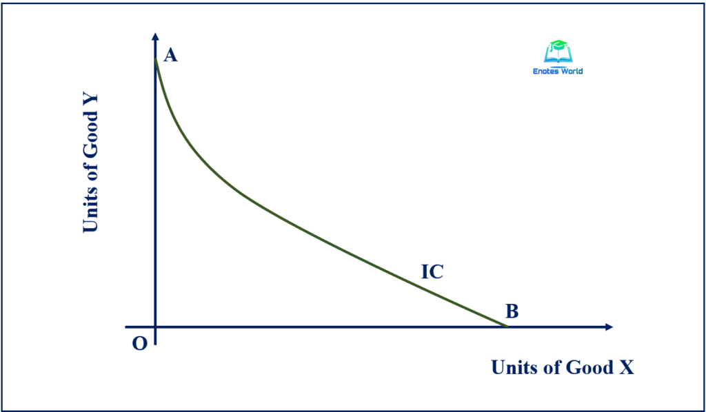
Derivation of Indifference Curve
If we plot the indifference schedule into the graph, we get the indifference curve. Hence the graphical exhibition of the indifference schedule gives an indifference curve. The following graph shows the graphical presentation of the above indifference schedule.
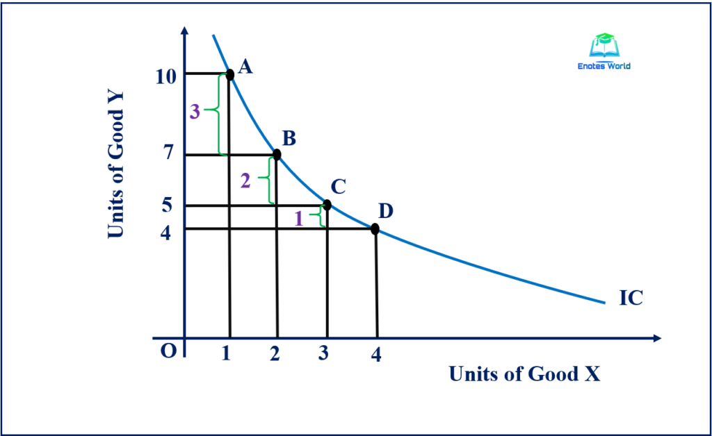
In the above figure, the quantity of good X is measured along the X-axis, and the quantity of good Y is measured along Y-axis. IC is the indifference curve which shows the different combinations of goods X and Y. All the combinations of both goods on the IC yield the same level of satisfaction to the consumer. Thus, if we take the locus of all these points, we get a curve showing various blends of at least two commodities that yields an equal level of pleasure to the buyers.
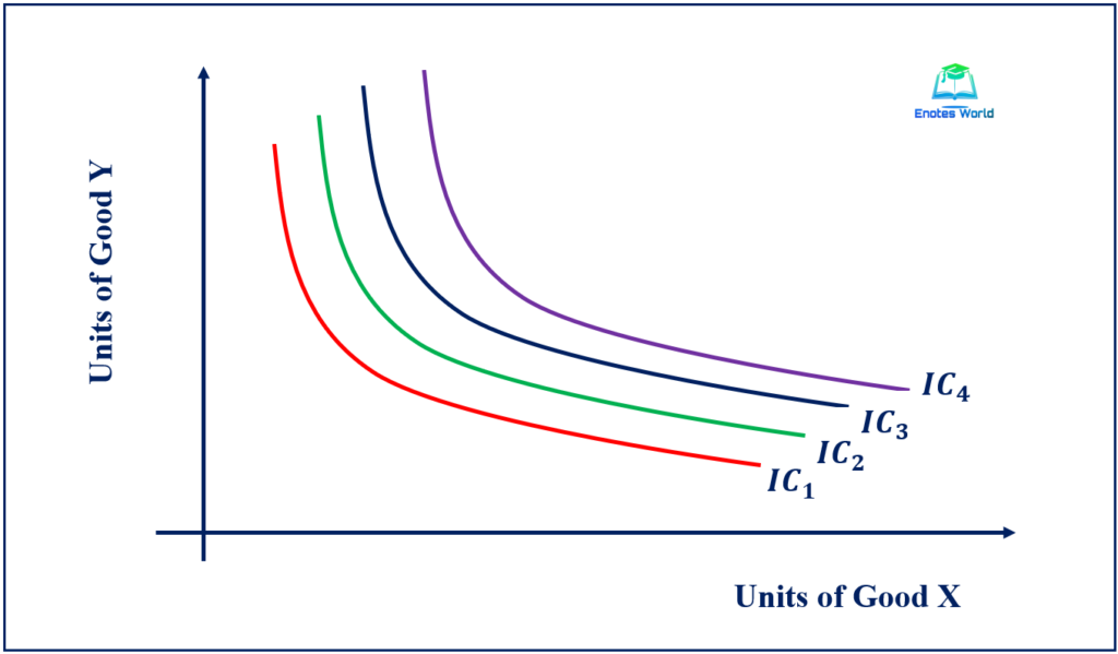
Indifference Curve Map/ Indifference Map
The assembly of various indifference curves in a graph is known as the indifference curve map. There are many indifference curves in the indifference map. Thus, an indifference map is a series of indifference curves for a particular consumer’s consumption of any two commodities. The buyer’s preferences can be completely described by an infinite number of ICs in the two-dimensional space, each IC representing a distinct level of satisfaction.
The upper indifference curve embodies a higher level of satisfaction than the lower indifference curve because if the consumer shifts to the right from one indifference curve to another, he obtains more of one or both commodities.
However, we have no hints on how much extra satisfaction or utility an upper indifference curve directs. An indifference curve far away from the origin is higher or the upper indifference curve close to the origin is a lower indifference curve. The following figure is a set of ICs. This is called an indifference map.
Properties/ Features/ Characteristics/Standard of Indifference Curve
The major properties of the indifference curve are as below;
The Indifference Curve is Negatively Sloped
The indifference curve is generally downward sloping. This is an important feature of the IC. When a consumer desires to have more of a commodity, then the quantity of other commodities declines so that he remains on the same level of satisfaction. This is possible only when the indifference curves slope downward from left to the right. Therefore, downward sloping IC implies that the two goods are a substitute for one another but not a perfect substitute. The following figures show the downward-sloping indifference curve;
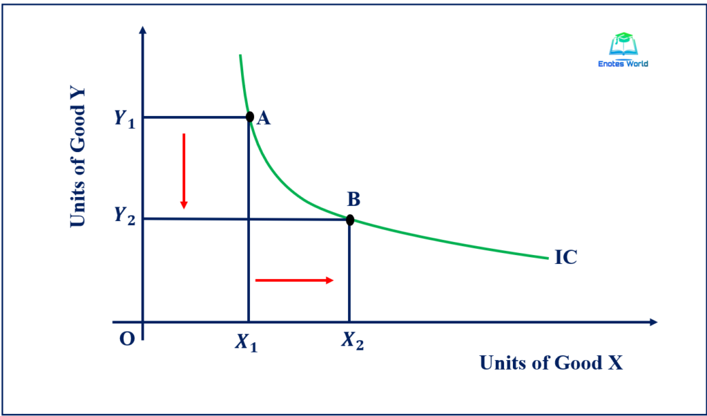
The above figure shows the downward-sloping indifference curve. When the consumer moves from point A to B, the quantity of Y commodity decreases from Y1 to Y1, and at the same time, the number of X increases from X1 to X2 keeping the same level of satisfaction.
The Indifference Curve is Convex to the Origin
Indifference curves (ICs) are at all times convex to the origin due to the fact of diminishing marginal rate of substitution. The marginal rate of substitution of one commodity for another reduces or diminishes when more and more of one commodity is substituted for another. It means, the more we consume one commodity, the less we sacrifice another commodity so that IC is convex to the origin. The following figure shows the convex indifference curve.
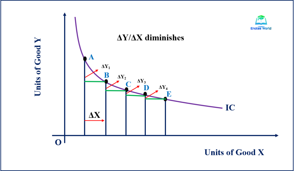
In the above figure we can say that if the consumer moves from A to B, he gives up ΔY1 of commodity Y to secure ΔX of commodity X. In this case, the MRSxy= ΔY1/ΔX. From the figure, it is clear that when he moves down from A to E, he gives up less and less of commodity Y for each additional unit of X. This fact shows a diminishing MRS.
Indifference Curves Do Not Intersect or Cross Each Other
Indifference curves cannot intersect with each other. If they intersect with each other then consumers’ choices won’t be consistent and transitive. Assume that we have IC1 and IC2 as two indifference curves. These two indifference curves characterize two different levels of satisfaction. If IC1 and IC2 cross or meet each other, that cross will denote a similar level of satisfaction, and that is impossible in IC analysis.
In the above figure, at point A, IC1, and IC2 intersect each other. Hence, at point A, both curves yield the same level of satisfaction. Observing such we cannot tell that which of these indifference curves gives higher satisfaction. It is not possible to answer in this case as two indifference curves cannot yield the same level of satisfaction.
The upper Indifference Curve Represents an Upper Level of Satisfaction
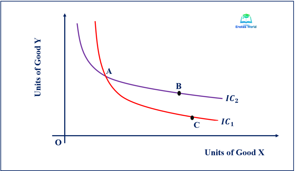
If we see the indifference map, we will see countless indifference curves. All these indifference curves signify the different amounts of pleasure. The higher indifference curve always expresses a higher level of pleasure and happiness to the consumer. A higher indifference curve that lies above and to the right of another indifference curve represents a higher level of pleasure and happiness and a combination of two goods on a lower indifference curve gives a lower level of happiness. The following figure helps to describe a such attributes of IC more clearly;
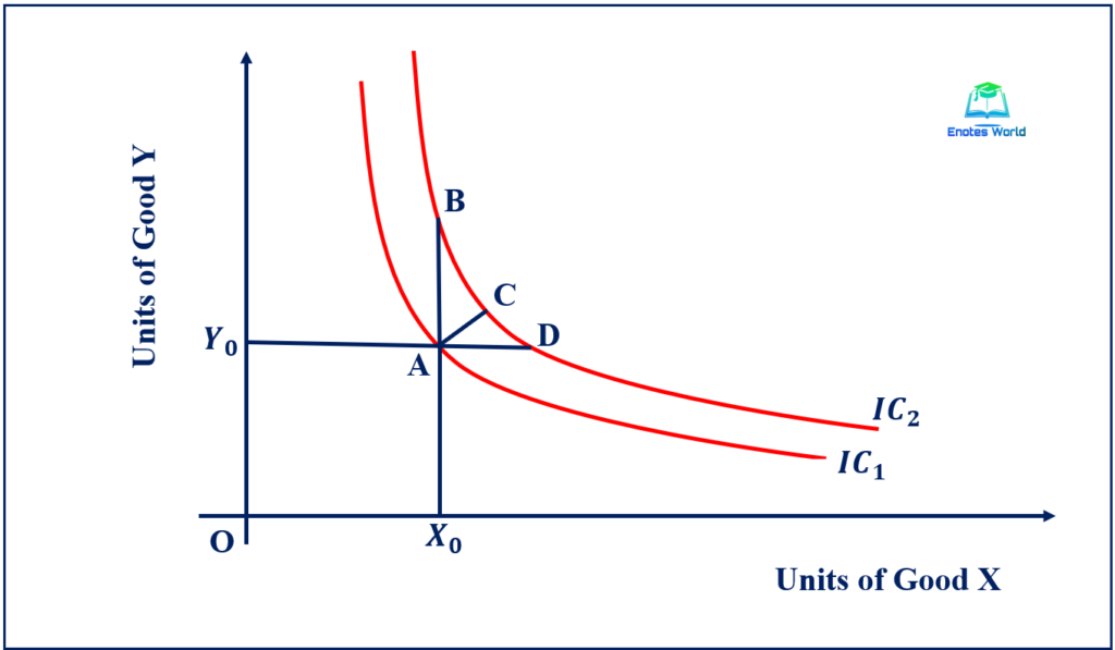
If a consumer shifts from point A to D as a horizontal shift, he gets a further amount of commodity X. The quantity of commodity X increases by ‘AD’ and the quantity of commodity Y remains the same (Y0). When he shifts from point A to B as a vertical shift, he gets more quantity of commodity Y. The quantity of commodity Y upsurges by ‘AB’ and the quantity of commodity X remains the same (X0). When the consumer shifts from point A to C (diagonal shift), he gets an additional quantity of both commodities (X and Y). Hence, an indifference curve to the right always embodies a higher level of fulfillment. Because of this reason, the consumer always attempts to move outward to maximize his level of satisfaction. This is recognized as the “monotonicity” of preferences.
Indifference Curves Never Touches Either or Both Axes
An indifference curve consists of various combinations of two merchandise. If an indifference curve traces the horizontal or vertical axis, it implies that the customer prefers only one commodity because when it touches axes, one of the commodities becomes zero in quantity. This interrupts the basic explanation of an indifference curve. Hence, an indifference curve does not touch either a horizontal axis or a vertical axis.
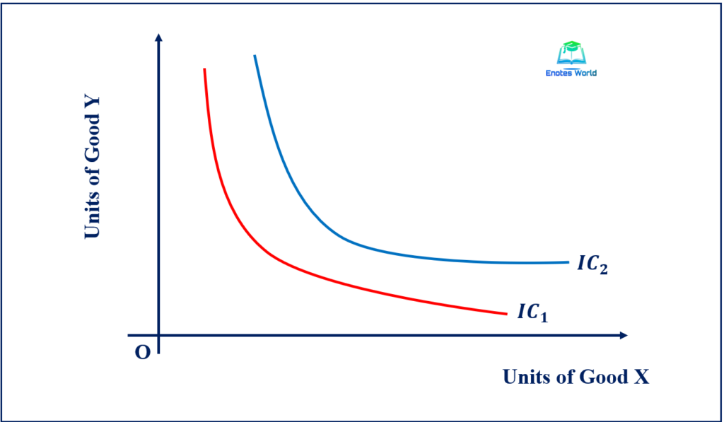
Indifference Curve Need Not be Parallel With Each Other
Indifference curves are declining negatively sloped from the left to the right but the rate of sacrifice for different consumers may differ and as a result indifference curves are not parallel to each other. It means every indifference curve may have a different diminishing marginal rate of substitution between the goods. Hence it is not necessary that two indifference curves must be parallel as shown in the following diagram;
Conclusion
Indifference curves are a key tool in economic analysis because they are used to represent an ordinal measure of the tastes and preferences of the consumers and to show how the consumer maximizes utility in spending income. The theory was developed so that analysis of economic choice could be used for preference, which can be observed, rather than the older concept of utility. It represents the same level of satisfaction of a consumer from different bundles of commodities i.e. the satisfaction or pleasure that a consumer can get leftovers the identical lengthways of an IC. The above assumptions and properties of the indifference curve have explained its concept clearly.
References and Suggesting Readings
Ahuja, H.L. (2017). Advance Economic Theory. New Delhi: S. Chand & Company.
Dhakal, R. (2019). Microeconomics for Business. Kathmandu: Samjahan Publication Pvt. Ltd.
Dwivedi, D. N. (2018). Microeconomics Theory and Application. New Delhi: Vikas Publishing House PVT LTD
Kanel, N.R. and et. al. (2019). Microeconomics for Business. Kathmandu: Buddha Publications.
Shrestha, P.P. and et. al. (2019). Microeconomics for Business. Kathmandu: Advance Saraswati Prakashan.
very productive work. it has been helpful to me