A supply curve is a diagrammatic presentation of the law of supply. It delivers the same information as a supply schedule does. The supply curve is a geometric expression of the schedule showing a positive relationship between the price of the commodity and its supply. The supply curve is derived based on the same assumptions of the law of supply and supply schedule. Like the supply schedule, the supply curve is also of two types as individual and market supply curve.

Individual Supply Curve

It can be defined as the curve that shows various quantities of a commodity that an individual producer or supplier is willing to supply at different prices during a given time, assuming other factors affecting supply remain unchanged. In a simple sense, it is the graphical presentation of the individual supply schedule. Thus, it shows the various quantities of supply of a commodity by a particular firm at various prices. Its alternative name is a single producer’s supply curve. The following table and the corresponding graph show the individual supply schedule and individual supply curve respectively.

Price (Rs. Per Unit)	Quantity Supplied (Units)
20	10
40	20
60	30
80	40
100	50

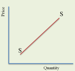
The table shows various prices of the product and the corresponding supply of the producer. This supply schedule explains the law of supply, a direct relationship between price and supply. The following graph shows the individual supply curve;

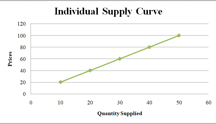
The above figure is the graphical transformation of the individual supply schedule. The positively sloping supply curve shows the direct relationship between the price and quantity supply.

Market Supply Curve

The market supply curve can be defined as the curve that shows various quantities of a commodity that all the producers or sellers or suppliers are willing to produce and sell at different prices during a given time, holding other factors affecting supply constant. It shows the various quantities of supply of a commodity of the whole market at various prices. Geometrically it is the horizontal summation of all the individual supply curves. It also slopes upwards, left to right showing a direct relationship between price and market supply.

It can be derived with the help of a market demand schedule. Let us assume there are only three suppliers namely supplier A, B, and C of a particular product during given specific time.  The following table shows the market supply schedule and the corresponding figure shows that the market supply curve or derivation of the market supply curve.

Price	Supply of A	Supply of B	Supply of C	Market Supply(A+B+C)
200	1	2	3	6
400	2	4	6	12
600	3	6	9	18
800	4	8	12	24
1000	5	10	15	30

The above table shows various units of a commodity supplied by three different suppliers. When the price of a product increases their supply also increases and vice versa.  The following figure shows the derivation of the market supply curve.

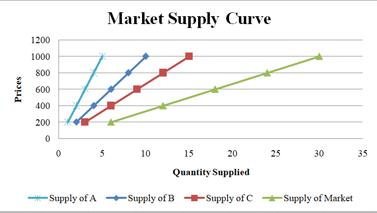
In the above figure, the initial three upward-sloping supply curves are the individual supply curve for supplies A, B, and C respectively. The flatter fourth supply curve is the market supply curve. By adding horizontally all the individual supply supplies at each price level, we get the market supply curve. The upward-sloping market supply curve exhibits that price and market supply positively move.

Alternative Method

Instead of showing individual supply and market supply in a single graph, we can also show them by drawing in a separate graph. The following figure shows the alternative representation of individual and market supply curves.

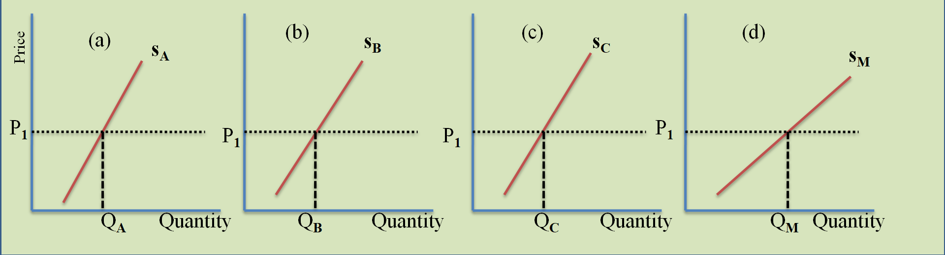
Figure (a) shows the individual supply curve of supplier ‘A’, figure (b) shows the supply curve of supplier ‘B’, and figure (c) shows the supply curve of ‘C’. By adding all the individual supply horizontally at the given level of the price we get market supply curve S_M which is drawn in figure (d). For example, at price P₁, Q_M=Q_A+Q_B+Q_C. The upward-sloping market supply curve conveys that price and market supply are positively related.

Difference between Individual and Market Supply Curve

Both the individual and market supply curves slope upwards and both establish a positive relationship between the price and supply of a commodity. However, the following differences are there between the individual and market supply curve.

1. Individual supply curves are nearer to the origin but the market supply curve is farther from the origin or market supply curve is flatter than individual supply curves.
2. The nature of the supply curve of the individual seller is individual, but the market supply curve is the horizontal summation of all the individual supply curves.
3. The individual supply curve shows the small quantity of supply for a commodity but the market supply curve shows the large volume of quantity supply of a commodity.

Supply and Time

Supply always responses to the change in price. But with reverence to time duration, the degree of response may change. We may divide time into the following three periods on such a basis.

Market Period

It is a very short period and in this period the supply is fixed. The maximum supply in the market period is the stock of the good which has already been produced. This is the case of the supply of perishable goods. For example, once the birthday cake is produced and brought to the market, there cannot be any change in the supply of cake, no matter what the price is. Therefore, in the market period firms cannot adjust their output to any change in the price. Thus the supply curve of the firm is vertical. The diagram below shows the nature of the supply curve;

Sort-Run

The short-run is the period in which supply can be adjusted to some extent. Producers in the short-run can increase production only by operating the active plant for longer hours like double shifts instead of one shift. The short-run period is not long enough for the firms to set up new plants or new machines. Thus, short-run supply can be increased to a limited extent. The short-run supply curve is upward sloping and steeper curve as shown in the following figure.

Long-Run

It is the time during which the firm can build new plants or close down the old plants. Moreover, new firms can enter the industry by setting up new plants. Therefore, it is possible to bring about a large change in quantity supply in the long run. The supply curve, in the long run, is flatter as shown in the following diagram.

Exceptions to the Upward Sloping Supply Curve

Generally, the supply curve is upward sloping showing the direct relationship between price and supply, holing other things remaining constant. However, in certain exceptional cases, the supply curve may take a different shape that we mention earlier. The following situation reveals the different shapes of the supply curve. 

Vertical Supply Curve

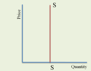
In the case of certain commodities, the supply curve may be a vertical one. Especially when the commodity is of such a nature that cannot be increased or decreased at all then the supply curve will be vertical. For example, classical painting, old manuscripts, rare postage stamps, old coins, etc are fixed in supply. Similarly the supply of agricultural products etc. also cannot be increased in the short-run so supply remains fixed. The supply of sheets in the stadium is also fixed in the short-run. In these all cases, the supply may be fixed and the curve will become vertical one as shown in the following diagram.

Backward Bending Supply Curve

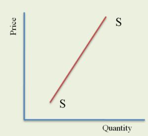
The supply curve may be backward bending also. This means a smaller quantity will be supplied at a higher price than a lower price. The following figure shows the backward sloping supply curve.

In the above figure when the price is OP, the supply of the product is OQ₁. When the price increases to OP₁ from OP, the supply is decreased from OQ to OQ₁. As a result, the supply curve SS becomes negatively sloping after point T. Such type of backward bending supply curve may occur in case of labor supply. Initially, the worker offers more hours of working with an increase in the price of labor but after a certain level, the worker prefers more leisure time even at a higher wage rate. At a very high wage rate, the worker prefers leisure to work as he may have earned enough income.

Conclusion

Therefore supply curve is a graphical presentation of various combinations between price and quantity supply that are positively related to each other. The individual as well as market supply curve generally slope upward from left to the right because as higher prices sellers are willing to sell more as higher price brings more profit margins. Moreover, because of economies of scale, it is profit worthy for suppliers to produce more and supply more because per unit cost of production with large production will decrease. In some special cases, the shape of the supply curve may be vertical as well as backward bending also.