Besides the analysis of consumer behavior and consumer demand, the technique of the indifference curve can be used in the analysis of several other economic phenomena and issues. Mainly the technique of indifference curves is applied in the areas like consumer’s surplus, the individual labor supply curve, numerous doctrines of welfare economics, the burden of different forms of taxation, gain from foreign trade, welfare implications of subsidy provided by the government, index number problems and so on. Here we will explain the use of the indifference curve technique on taxation (direct vs indirect taxation) and income-leisure choice of the people (application and uses of indifference curve).  

Application and Uses of Indifference Curve in Measuring Welfare Effect of Direct and Indirect Tax

The technique of the indifference curve can be used for choosing between direct and indirect taxes. The use of the indifference curve will help to judge the welfare effect of direct and indirect taxes on the individuals. If the government is eager to raise the tax revenue and at that time the government may face the issue regarding whether it will be better to do so, imposing a direct tax or an indirect tax from the viewpoint of the welfare of the individuals. Thus, policymakers are often faced with a problem; what tax to impose to raise revenue at minimum social cost-income tax or excise duty.

In general, income tax is preferable over indirect tax (direct tax is profitable over indirect tax from the viewpoint of social welfare) as a source of public revenue. Thus, here we will show that indirect tax such as excise duty causes an excess burden on the individuals (indirect taxes reduce the people’s welfare more than the direct tax) than the imposition of direct tax if the government has to increase the equal amount of revenue through them. 

The following figure with the help of the indifference curve shows the relative burden of income tax and excise duty.

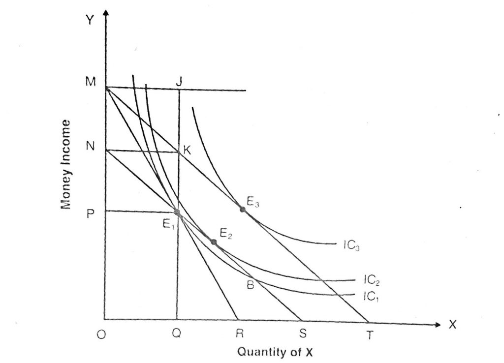
Suppose that an individual has an OM level of money income shown by budget line MT in the above figure. The individual spends his total income on commodity X. With no taxation of the government, the consumer is in the equilibrium at point E₃ on the indifference curve IC₃.  Now let us assume that the government imposes excise duty on commodity X, and as a result, its price increases and the budget line MT swings to MR. With a swing in the budget line consumer’s equilibrium establishes on a lower indifference curve at point E₁.

At the point E₁, the consumer buys OQ units of good X and pays MP=JE₁ income for it. In the absence of excise duty, the OQ amount of good X could purchase by the consumer at the income of JK=MN. Thus, the difference between the two JE₁-JK=KE₁ is excise duty.

Let us again assume that the government imposes income taxes, instead of excise duty, on the individual at the condition of equilibrium E₃, on the TC₃ to raise the same amount of revenue (KE₁). As a result, the price line shifts leftwards as parallel from MT to NS that passes through the point E₁.  With the price line NS now, the consumer is in equilibrium at point E₂ on the indifference curve IC₂, which lies at a higher level than IC₁. Here the income tax (MN) is equal to excise duty (KE₁). Thus, income tax of equal amount places the consumer on a higher indifference curve (IC₂) than does the excise duty (IC₁).

This is so because an excise tax, that alters the price structure, enforces both substitution and income effects on the consumer’s choice whereas income tax enforces only income effect. As a result, an excise duty reduces consumer satisfaction due to both income and substitution effects whereas income tax reduces it only to the extent of the income effect. Thus, a direct tax is superior in the choice between direct tax versus indirect tax in policymaking.

Application and Uses of Indifference Curve in Measurement of Effect of Excise and Income Subsidies

One of the applications of the indifference curve is to analyze with its aid the effect of subsidies to the consumers. The government provides several types of subsidies to people to promote their welfare. Here we will compare the effect of excise and income subsidies as policy measures by the government. 

Suppose that the government is planning to boost the living standard of poor people by providing subsidies and has to choose between income subsidy in the form of lump-sum money grant, and excise subsidy or subsidy in the form of food subsidy, rent subsidy, and loan subsidy. Here, we have to analyze the cost of each type of subsidy to the government and the profitability to the people. The application of the indifference curve technique will help us to define and decide on the given issues.

Let us assume a simple situation of choosing between an excise subsidy on a commodity X and a lump-sum subsidy, granted to a single consumer. The following figure helps us to analyze both of the policy options in a profitable manner.

Measuring Financial Cost of Excise Subsidy

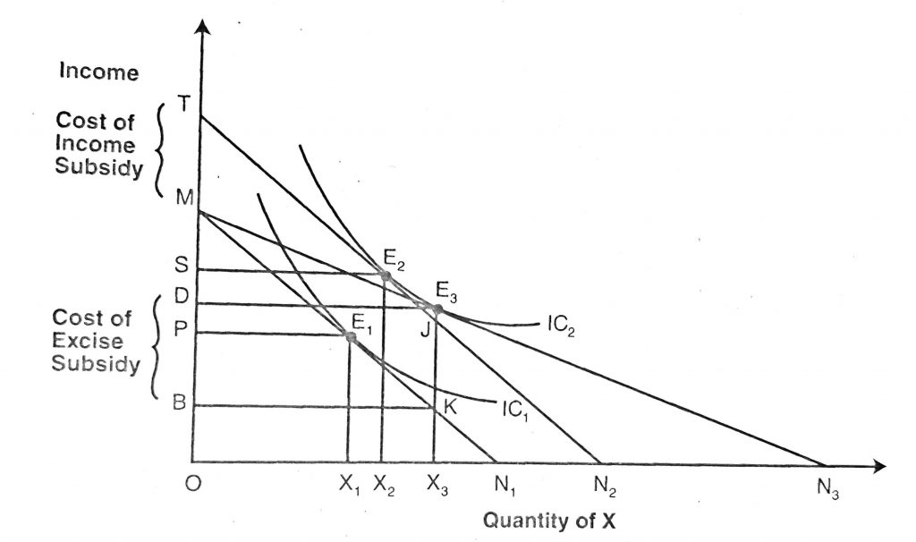
Suppose the budget line of the consumer is MN₁ and the indifference curves are IC₁ and IC₂. Given the income and price of commodity X, the consumer is initially in equilibrium at point E₁ on IC₁. At the equilibrium point, he consumes OX₁ units of good X and pays MP of his money income and retains OP for other goods.

The government provides excise subsidy and as a result, the commodity X subsidizes by 50 percent of its price so that the price of the commodity X falls to a half. With a fall in price, the budget line MN₁ swings to MN₃ such that ON₁=N₁N₃. The consumer moves on to equilibrium point E₃ from E₁. At the new equilibrium point E₃, he consumes OX₃ units of good X and pays DM of his income at the subsidized price. With no excise subsidy, the consumer would have paid MB of his income to get OX₃ units of good X. Thus MB-MD= DB is the cost of excise subsidy that the government would pay to the producers of the commodity.

 

Measuring Financial Cost of Lump-Sum Income Subsidy

Now let us consider that the government wants to replace the previous excise subsidy by the lump-sum income subsidy. The financial burden of income subsidy to the government is also analyzed with the help of the indifference curve presented in the above diagram.

Suppose that the government provides income subsidy just identical to excise or price subsidy. It means income subsidy is just sufficient to maintain the consumer’s level of satisfaction equivalent to price subsidy.  To observe the effect of income subsidy, let us assume that the government has provided income grants so that the budget line shifts parallelly from MN₁ to TN₂. The shifted line is tangent with higher indifference curve IC₂ at point E₂. At the new equilibrium point E2, the consumer buys OX₂ units of good X and pays TS of his income including income subsidy. Here in TS amount of total income, TM is the income subsidy provided by the government. So, the cost of income subsidy to the government is equaled to TS-MS=TM.

Comparing the cost of these two types of subsidies, we get

Cost of excise subsidy: DB=E₃K and

Cost of income subsidy: TM=JK

From the figure we can see that, E₃K>JK, so that the cost of excise subsidy(E₃K) is higher than the cost of income subsidy (JK). Therefore, we can conclude that the cost of subsidy E₃K is greater than the income subsidy JK though both the policy measures achieve the same goal of boosting consumers’ satisfaction to the level indicated by the indifference curve IC₂.

Therefore, income subsidy is more efficient from the consumer’s viewpoint and social cost viewpoint. However, the level of consumer satisfaction under both subsidy scheme is the same.  

Application and Use of Indifference Curve in Income-Leisure Choice

Another use of the indifference curve technique is that it is applied in the selection of income-leisure choice of the workers. To explain the choice of income-leisure let us assume a given utility function of an individual worker is;

U= f (M, L)

Where M stands for money income from work and L stands for leisure and entertainment.    

Assume that an individual worker divides his daily time between work and leisure to maximize his utility objective. Since the number of hours per day is fixed so increase the hours for work will reduce the hours available for leisure and vice versa. For labor, income and leisure are like a substitute for one another. A utility-maximizing worker sets the combination of work and leisure that maximizes his total utility function.

The following figure helps to see how labor makes his choice between leisure and income to maximize his utility function with the help of the indifference curve technique.

 

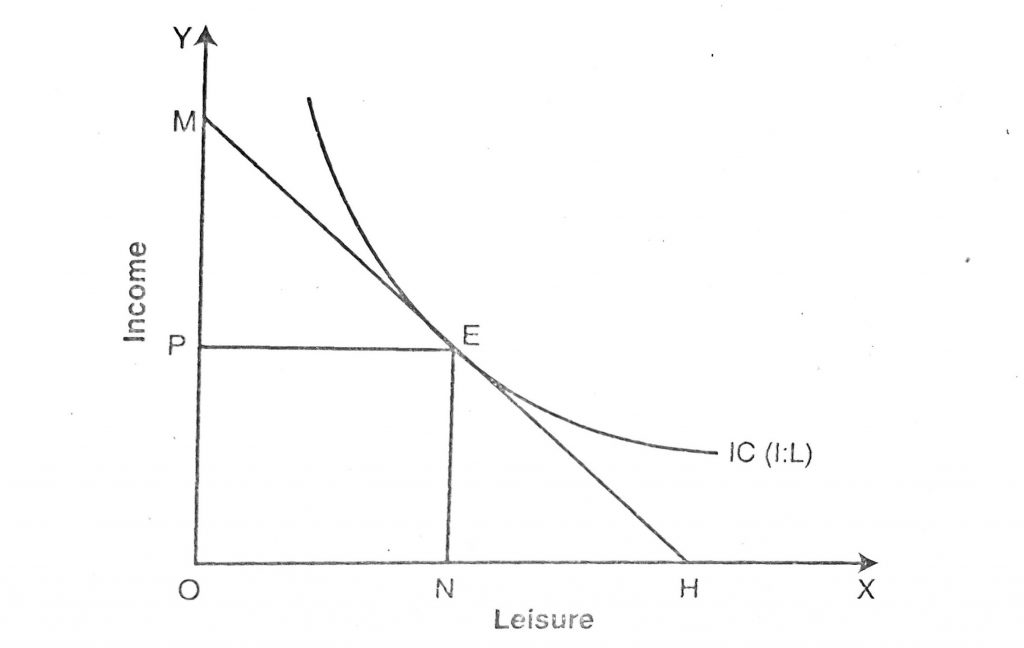
In the above figure, the x-axis measures the leisure time and the y-axis measures the income from work. Assume that OH displays the total hours available to the worker and hourly wage rate us W. if the worker works for OH hours and enjoys no leisure, his total income is OM. If the worker enjoys his whole time OH as leisure, he will be at point H with zero income. By joining these two extreme points M and H by a line, we get an income-leisure line, MH. It is also known as an income-leisure budget line. This curve shows many combinations of income and leisure. The curve shows various combinations of income and leisure at wage rate W and the slope of the line is OM/OH=W.

 Let us again assume that the income-leisure indifference curve of an individual is given by the curve IC in the figure and this curve is also known as the income-leisure trade-off curve. The slope of this curve MRS _{L, M}. is a marginal rate of substitution between income and leisure and it is ΔM/ΔL.

The worker’s equilibrium is measured at point E where the income-leisure line is tangent to his income-leisure trade-off curve. It means the slope of the income-leisure line is equal to the slope of the income-leisure trade-off curve.

So, at point E; W= ΔM/ΔL=MRS _{L, M}  

Point E in the figure shoes worker’s optimal combination of income and leisure with the OP of income and ON hours of leisure. Here worker has to work {Total hours (OH)-Leisure hours (ON)=NH} NH hours to earn EN level of income. This combination holds only at the wage rate of W per hour.  When there is an increase or change in wage rate per hour, the equilibrium combination of income-leisure will go change.

References and Suggested Readings

Acharya, K.R. (2018). Microeconomics. Kathmandu: Asmita Books Publishers & Distributors (P) LTD.

Ahuja, H.L. (2017). Advance Economic Theory. New Delhi: S. Chand & Company.   

Dwivedi, D. N. (2018). Microeconomics Theory and Application. New Delhi: Vikas Publishing House PVT LTD