Learning Objective To explain the derivation of the demand curve with help of the price consumption curve (Price effect and derivation of the demand curve)

The price effect is defined as the change in quantity demanded of a commodity due to a change in its price, assuming the price of other goods and the income of the people remain the same. The change in the price of the commodity has a direct effect on the consumer’s demand for that commodity. When there is a decrease in the price, the real income of the consumer rises, and that leads to a rise in the purchasing power of the consumer. As a result, the budget line swings towards the right, and the consumer will obtain equilibrium at the upper indifference curve.

Likewise, if there is a rise in the price then it will reduce the consumer’s purchasing power, and the budget line swings to the left signifying less quantity of purchase by the consumer. Joining different equilibrium points, we obtain the price consumption curve and with the help of the PPC, we can derive the demand curve for the product (price effect and derivation of the demand curve). Here we will derive the demand curve of a normal good with the help of a price consumption curve.

Case-I: When Two Goods Are Normal and Substitutable

The derivation of the price demand curve in the case of normal and substitutable goods is shown with the help of the following diagram.

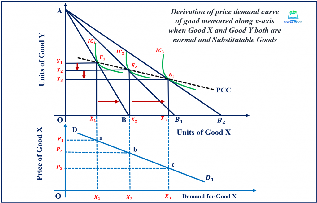
In the above figure, the upper part shows the derivation of the price consumption curve for substitutable normal goods and the lower part shows the derivation of the price demand curve. In the upper section of the figure, AB is the initial budget line and tangent with the indifference curve IC₁ at point E₁ showings X₁ and Y₁ units of consumption by the consumer.

Suppose there is a fall in price, as a result of the real income of the consumer increasing so that the consumer attains equilibrium at different prices and different higher ICs. In the figure, the consumer has shifted from E1 to E2 and from E2 to E3 with a fall in the price of good X and increased the demand for good X continuously from X1 to X2 and from X2 to X3 respectively. Since good X and Y are substitutable goods, with an increase in demand for good X, the buyer has reduced the demand for good Y from Y1 to Y2 and from Y2 to Y3 respectively. By joining these equilibrium points in the upper section, we got a downward-sloping curve which is known as the price consumption curve.

Based on such PCC, the price demand curve for good X can be derived as shown in the second part of the diagram. Quantities of good X are copied from the upper part of the diagram. The equilibrium point E₁ gives the combination of price P₁ and X₁ demand for good X and is shown by the combination in the second part of the figure.  Similarly, equilibrium points E₂ and E₃ have helped to get the combination b and c in the lower section of the graph. Joining the combination, a, b, and c, we get the downward sloping price demand curve DD₁ showing an inverse relationship between price and demand for good X.

Case-II: When Two Goods Are Normal and Complementary

The following figure helps to show the derivation of the price demand curve in the case of normal and complementary goods.

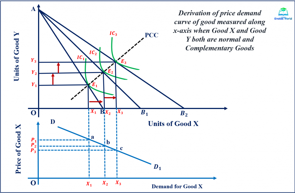
In the above figure (upper part), the derivation of the price consumption curve and derivation of the price demand curve has shown (lower part). In the upper part of the figure, we see that with a fall in the price of good X, the budget line continually swings from AB to AB₁ and from AB₁ to AB₂ and the consumer obtained his equilibrium accordingly at points E1, E2, and E3 respectively. When these equilibrium points are joined, we get an upward-sloping price consumption curve showing the increase in demand for good X and good Y both in case of a fall in the price of good X, assuming the price of good Y and money income available to the buyer remains the same.

In the lower part of the figure, the price demand curve for good X has been derived. The quantities of good X are copied from the upper part of the figure and the price of good X has shown along with the Y-axis. Based on the PCC derived in the upper part of the figure, the demand curve in the lower part has been derived.

The equilibrium point E₁ of the upper part gives the combination of price P₁ and quantity X1 of good X and is shown by the point ‘a’ in the lower section of the graph. Similarly, we get the combination of price and quantity with the help of equilibrium point E2 and E3 and denote by point b and c in the lower section of the graph. If we join points a, b, and c, the downward-sloping price demand curve DD₁ for good X has obtained in the lower part of the graph.

Case-III: When Two Goods Are Non-Related

The following figure shows the derivation of the price demand curve in the case of non-related two goods. Here we will derive the demand curve for normal goods measured along the x-axis when goods measured along both axes are non-related to each other.  

The upper part of the figure has shown the derivation of the price consumption curve and with the help of PCC, the derivation of the price demand curve is shown in the second part of the figure.

Initially, the consumer was in equilibrium at E_1, and with a decrease in the price of good X, the consumer attains equilibrium at E2 and E3. If we join all three equilibrium points, we get PCC which is horizontal indicating that the quantity of X is increased from X1 to X2 and X3, and the quantity of Y remains constant at Y1. This shows that goods X and Y are non-related goods.

Based on the upper part of the figure, the price-demand curve for good X is derived in the lower part of the figure. At the equilibrium point E₁, we see that X₁ units of good X and Y1 units of good Y are demanded by the consumer at the P₁ price of good X. With a continuous fall in the price of good X, the consumer attains equilibrium E₂ and E₃ and consumes X₂ and X₃ units of good X and Y₁ units of good Y.

With the help of equilibrium point E₁, E_2, and E3, we get the price-quantity combinations of good X as shown by point a, b, and c in the lower part of the diagram. By joining these combinations, we get the downward-sloping demand curve DD₁ of good X.    

References and Suggesting Readings

Acharya, K.R. (2018). Microeconomics. Kathmandu: Asmita Books Publishers & Distributors (P) LTD.

Ahuja, H.L. (2017). Advance Economic Theory. New Delhi: S. Chand & Company.   

Dhakal, R. (2019). Microeconomics for Business. Kathmandu: Samjahan Publication Pvt. Ltd.