Economics through its different theories and principles help to economic agents and participants in their decision-making processes and help them to get their objective fulfilled. For instance, a manager may have to think of what level of output he has to produce. Managers will produce the level of output that maximizes the form’s profit if he has set the objective of profit-maximizing. Likewise, he may have to go for selecting the least-cost mixture of factors to manufacture the best possible level of output. Thus, to produce a profit-maximizing level of output he will have to choose the combination of inputs that minimizes the cost of producing a given level of output. Here we will talk about basic mathematical concepts used in economics.
In recent times, the use of mathematical analytical tools and models has become a popular and regular phenomenon in economic research and business decision making. Mathematical formulations of analytical models of decision-making are expressed in terms of functions that describe the economic relationship between various variables. Here we discuss the basic mathematical concepts needed to understand the relationship between economic variables and to make business decisions.
Contents
Functions
A function explains the association stuck between two or more variables. Thus, a function presents the dependence of one variable on one or other variables. If the value of a variable Y depends on another variable like X, we can write,
Y=f (X)……………. (i)
Where f stands for functional relation
The function (i) is read as ‘Y is a function of X’. It means that each value of the variable Y is accounted for by a distinctive value of the variable X. Y is the dependent variable and X is the independent variable. The independent variable is also considered as a cause and the dependent variable as an effect. The demand function is one of the widely used functions in economics. The demand function expresses the quantity demanded of a commodity is a function of its price, ceteris paribus. Thus, demand for a good X is described as under;
DX=f (PX)
Where DX is the demand quantity of commodity X and PX is its price.
Similarly, the supply equation of a commodity X is displayed as;
SX=f (PX)
When the value of the variable Y relies on more than two variables X1, X2…Xn then such function can be expressed as;
Y=f (X1, X2, X3 …Xn)
This shows that the variable Y depends on several independent variables X1, X2, X3 …Xn where n is the number of independent variables. For example, demand for a product is generally considered to be a function of its price, price of other goods, the income of the consumer’s, tastes and preferences of the consumers and advertisement expenditure, etc. Thus,
DX=f (PX, PY, M, T, A)
Where DX is a demand for the commodity X; PX is the price of the commodity X; PY is the price of a substitute product Y; M is the income of the consumer; T is the tastes and preferences of the consumers for the product, and A is advertisement expenditure incurred by the firm.
The accurate number of the relation of the dependent variable with the independent variables can be known from the specific form of the function. The specific form of a function can be taking a variety of mathematical forms. Here we will discuss some specific types of function.
Linear Function
A broadly used mathematical form of a function is a linear function. It can be spoken as;
Y = a + bX
Where ‘a’ and ‘b’ are positive and known as parameters of the function. We know that the parameters of a function are variables that are fixed and given in a specific function. The values of constants ‘a’ and ‘b’ decide the precise character of a linear function. The linear demand function having price only as an independent variable is expressed as;
Qd = a-bP
Here the negative sign before ‘b’ displays that the quantity demand of a product is negatively connected with the price of that product. If ‘a’ equals 7 and ‘b’ equals 0.5, then the linear demand function can be written in the given specific form:
Qd = 7 – 0.5 P
The given specific demand function tells that a unit drop in the price of the product, there will increase in the demand quantity by 0.5 units. If the price is zero, then the term (0.5P) in the demand function will also account zero and the quantity demanded is equal to 7.
We can consider different values of P and find out the different values of quantities (Qd) of a product demanded at them. In the following figure, different price-quantity combinations are shown derived from the demand function Qd = 7 – 0.5P
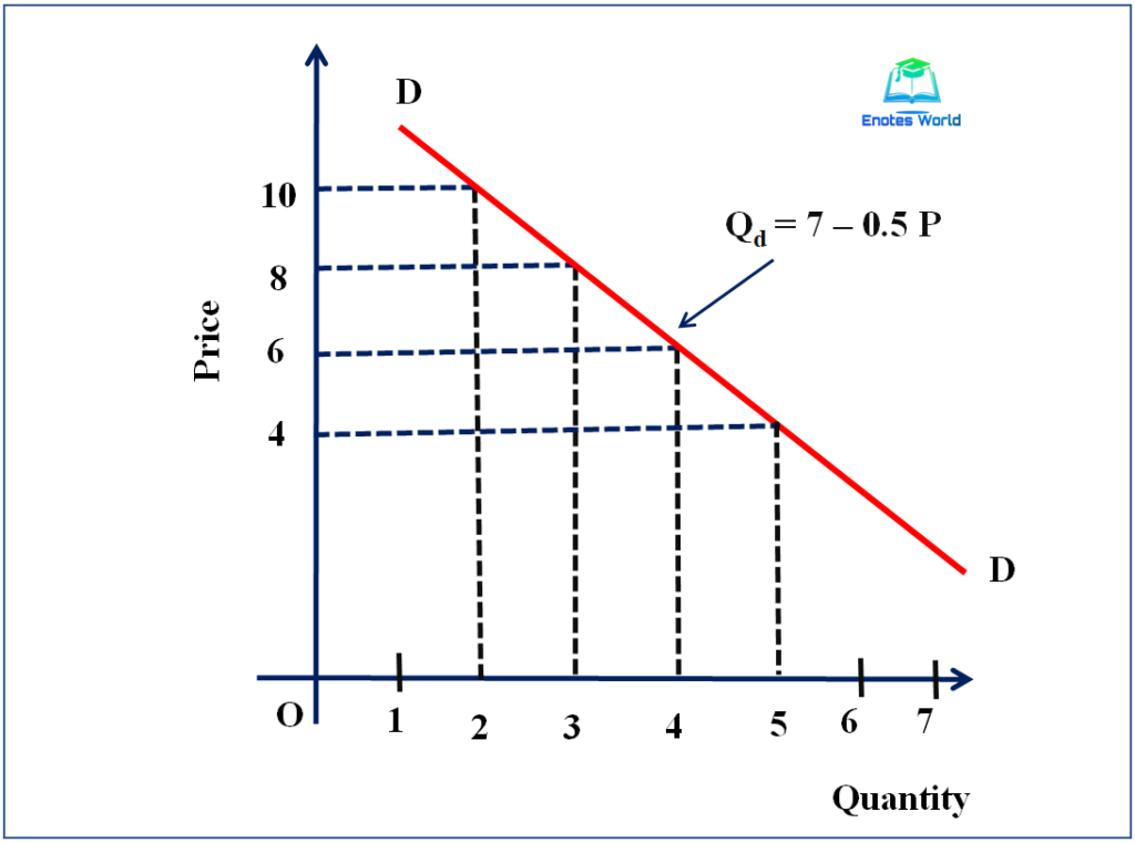
It should be noted that in economics to represent demand function we demonstrate the independent variable (price in the above case of demand function) on the y-axis and the dependent variable (the quantity demand) on the x-axis. The graph of linear demand function has shown by the above graph. If we signify quantity demanded (Qd) on the y-axis, and price (Px) on the x-axis the slope of the demand curve so drawn would be equal to ∆Q/∆P.
Multivariate Linear Demand Function
The linear demand function having two or more than two independent variables is a multivariate linear demand function. The following function displays the multivariate linear demand function;
Qx = a + β1 PX + β 2 PY + β 3 M + β 4 T + β 5 A
Where β 1, β 2, β 3, β 4 are the coefficients of the particular variables. In economics, we show the effect of determinants of demand other than the price of the product by the shift in the demand curve. For instance, when income (M) of the consumers goes up, consumers will demand more of the product X at a given price. This results in shifting the demand curve to the right from its original position.
The following equation shows the linear multivariate function;
Y = 6 – 0.5X1 + 0.3X2 + O.5X3 + 0. 45 X4
In the given function, 0.5, 0.3, 0.5, and 0.45 are coefficients and they demonstrate the unique shock of the independent variables X1, X2, X3, X4 on the dependent variable Y.
Power Functions
The linear functions discussed above are known as first-degree functions were the independent variables X1, X2, X3, etc have emerged to the first power only. Now we will explain power functions. The power functions of the quadratic and cubic forms are widely used in economic analyses.
Quadratic Functions
The function has one or more independent variables with degree two or power two is known as the quadratic function. The polynomial equation of degree 2 is called the quadratic equation. Power is also referred to as exponent. A quadratic function can be displayed as;
Y=a + βX + αX2
This signifies that the value of the dependent variable Y based on the constant a plus the coefficient β times the value of the independent variable X plus the coefficient α times the square of the variable X. Suppose a= 5, β = 4 and α = 3 then quadratic function takes the following specific form.
Y = 5 + 4X + 3 X2
We can get the changed values of Y for taking diverse values of the independent variable X.
Types of Quadratic Functions
There are two types of quadratic functions as convex quadratic functions and concave quadratic functions. The type or form of it depends on the sign of α, coefficient of X2. In the quadratic function Y=a + βX + αX2, if α is positive then it is known as a convex quadratic function because its graph is U-shaped. Similarly, if the sign of α is negative, that is a concave quadratic function because its graphs are of inverted U- shape. The following figure shows the shape of the concave and convex quadratic functions.
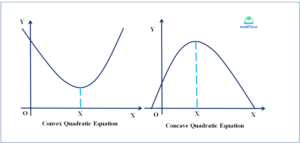
A quadratic function is plotted in a graph that gives a curve called parabola and the solution of the quadratic equation can be found with the help of parabola. Parabola is a curve having a turning point and changing slope at every point, unlike the linear curve.
Multivariable Quadratic Function
If there are two or more than two independent variables like X1, X2, and if they have a quadratic relationship with the dependent variable Y, then such a function is referred to as multivariable quadratic function. In the case of two independent variables X1 and X2 such a function may be displayed by below;
Y = a + βX1 – αX21 + גX2 – λX22
If the given function is graphically shown, it will be represented by a three – dimensional surface and not a two-dimensional curve.
Cubic Function
When the power function has a third-degree term relating to an independent variable then it is known as a cubic function. Thus, cubic functions may well have a degree first, second, and third-degree terms. The yardstick structure of the cubic function is;
Y= α+ βX + λX2 + גX3
Where the intercept term is α, and X is the predicted variable and X has the first second, and third-degree terms. When the signs of all the coefficients α, β, λ, and ג are positive, then the values of Y will increase by increasingly larger increments as the value of X increases.
However, when there are varying signs of diverse coefficients in the cubic function (it means a few have positive signs and some have negative signs), then the graph of the function may have both convex and concave based on the values of the coefficients. Such cubic function having different sign may be displayed as;
Y= α+ βX – λX2 + גX3
Slopes of the Functions
The rate of change at which variable changes in response to a change in another variable is known as a slope. For instance, the rate of change in quantity demanded of a commodity with the response to change in the price of a commodity. Here we will see the slope of linear as well as non-linear functions.
The slope of Linear Function
Consider the linear function as; Y=f(X) = 2+0.5X. Now we can compute different values of Y by considering different values of X such as 1,2,3,4 etc. The following table and graph show the different values of the variables based on the given linear function.
| Linear Function: Y=2+0.5X | ||||||
| Value of X | 0 | 1 | 2 | 3 | 4 | 5 |
| Value of Y | 2 | 2.5 | 3 | 3.5 | 4 | 4.5 |
The values are plotted in the graph as given below;
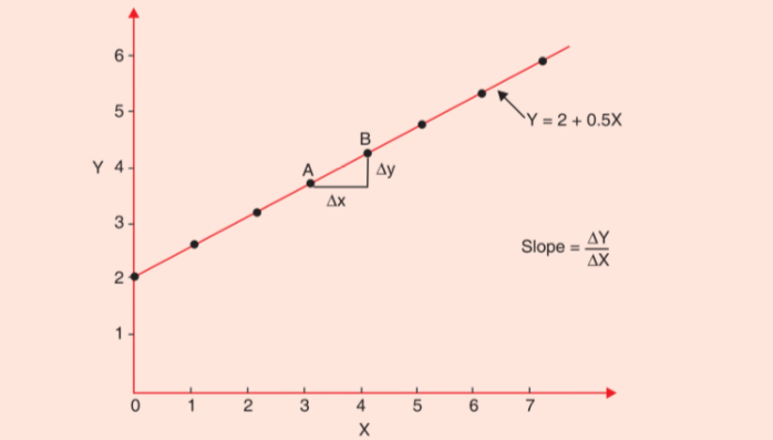
In the above figure, the measurement of the slope of linear function has been shown. The slope is measured by ΔY/ΔX. For example, at the point, A of the given function value of variable X is 3, and corresponding to it the value of Y is 3.5. When the value of X has increased from 3 to 4 then the value of Y will increase from 3.5 to 4. Thus, the slope of the function (Y=2+0.5X) is; ΔY/ΔX=4-3.5/4-3=0.5/1=0.5.
This implies that value of Y increases by 0.5 when the value of X increases by 1. The slope of a linear function is always the same at every point of the linear demand function.
The slope of a linear function can also be measured directly from the function itself. Consider the following linear function;
Y=a+bX
From the given linear function we can observe that, when X= 0, the value of Y= a. Thus, ‘a’ is Y-intercept. Further, in this function ‘b’ is the coefficient of X and measures change in Y due to change in X, which is ΔY/ΔX. So, ‘b’ represents the slope of the linear function. In linear function Y=2+0.5X, 2 is the Y-intercept, this is, the value of Y when X is zero. 0.5 is the value of ‘b’ that is the coefficient of X, which measures the slope ΔY/ΔX of the linear function.
The slope of the Non-linear Function
To explain the measurement of the slope of non-linear function let us consider a quadratic function Y= α+ βX – λX2 + גX3. If we plot the non-linear function into a graph we will get a non-linear curve. For better understanding let us consider the following quadratic equation;
Y=5+3X+X2
The following table shows the values of Y taking different values of X (0, 1, 2, 3, 4, 5, etc.)
| Quadratic Function: Y=5+3X+X2 | ||||||
| Value of X | 0 | 1 | 2 | 3 | 4 | 5 |
| Value of Y | 5 | 9 | 15 | 23 | 33 | 45 |
The data so obtained are plotted in a graph as shown by the following diagram;
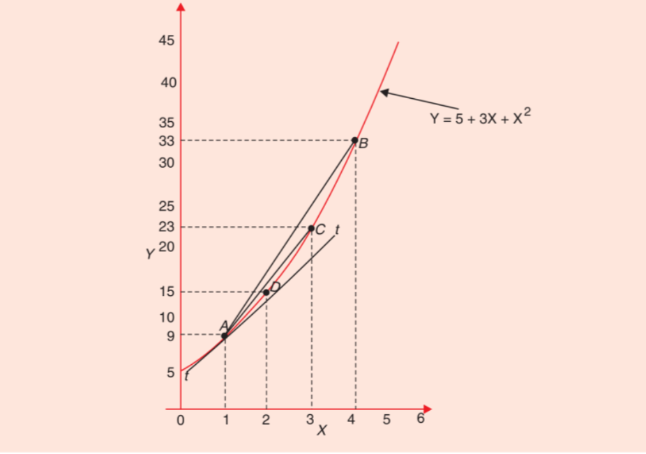
In the above figure, we see the measurement of the slope of line AB which connects two points A and B on a curve of a quadratic function can be measured by taking the changes in the value of Y divided by the change in the value of X. At point A, X=1, and the equivalent value of Y= 9 and at point B, X =4, and the analogous value of Y=33. Therefore, ΔX=3 and ΔY= 24. Here, thus the slope of the line AB is= ΔY/ ΔX=24/3=8
Similarly, the slope of straight-line AC in the above figure can be measured as, ΔY/ ΔX=14/2=7.
From the above calculation of slope, it will be seen that as ΔX decreases as it was 3 between A and B, 2 between A and C and 1 between A and B, the slope of the non-linear curve goes on declining. It was 8 of the line AB, 7 of the line AC, and 6 of line AD. As ΔX further decreases, the slope of the line connecting of the straight line connecting two points of the non-linear curve will further decline. Therefore, the slope at a point on the non-linear function curve can be measured by the slope of a tangent line drawn to the curve at that point.
References and Suggested Readings
Ahuja, H.L.(2017). Advanced Economic Theory. Delhi: S Chand and Company Limited
I like it. Very important points are included
Thank you! Keep supporting.