Introduction

In the analysis of consumer’s equilibrium, price and income are exogenous variables, and changes in the values of these variables have a direct effect on the consumer’s equilibrium or the consumer’s optimal choice of the goods. The effect of change in money income on the consumer’s optimal purchase decision is traced by the income consumption curve. Similarly, the price consumption curve traces the effect of change in price on the consumer’s equilibrium. In general, the change in price inversely affects the demand of consumers.

Holding the money income constant, if there is a fall in the price of the good, the consumer will be benefited due to the increase in the purchasing power and he or she can now purchase more units of goods, moving from the equilibrium point on the lower indifference curve to the equilibrium point on the higher indifference curve. Considering such types of change in exogenous variables and their effect on consumer’s choice we can derive the demand curve showing the relationship between price and quantity demand. Here, we will derive the ordinary/uncompensated/Marshallian and compensated/Hicksian demand curve due to the change in the prices of the product (Change in Prices and Derivation of Demand Curve).  

Meaning of Derivation of Uncompensated Demand Curve   

When there is a fall in the price of the commodity, there is an increase in the real income of the consumer, and if the consumer is not adjusted through compensation variation and he or she is demanding the units of good as a function of increased real income then the derived demand curve is the uncompensated demand curve. It means, in the case of the ordinary demand curve we include the substitution effect and income effect of change in the price of the good on the demand quantity.

Consumer moves to the higher indifference curve with a fall in the price in this case. Thus, the money income available to the consumer remains constant in case of the derivation of the uncompensated demand curve even after the decrease in the price of one good (good measured along with X-axis). This type of demand curve is known as the Marshallian or ordinary demand curve also.

Meaning of Derivation of Compensated Demand Curve    

On the other hand, when the demand curve is derived only considering the substitution effect of change in price on its quantity demand, then it is known as the compensated demand curve. It means while deriving the compensated demand curve the money income is compensated to keep real income constant (to keep satisfaction the same as before the change in price). For the proper and detailed analysis of consumer surplus types of issues, we better keep real income constant by reducing the money income (by the amount of compensation variation). Therefore, such a demand curve that incorporates the effects of change in the price of the good, real income remaining the constant is income compensated or compensated or Hicksian demand curve.

Derivation of Uncompensated and Compensated Demand Curve  

When we have to derive the uncompensated demand curve, the derivation procedure does consider the effect of both the substitution and income effect of the change in the price of the good, while the compensated demand curve only considers the substitution effect of price fall by keeping real income constant. Here we derive the ordinary and compensated demand curve of normal goods with a fall and rise in the price of the product (Change in Prices and Derivation of Demand Curve).

Case of Normal Good

If consumers demand more units with an increase in income and a fall in the price of goods then the good is called normal good. Income elasticity for a normal good is thus positive. We derive the demand curve of normal goods with the conditions of fall and rise in the price of the good.

Derivation of Ordinary and Compensated Demand Curve for the Fall in Price

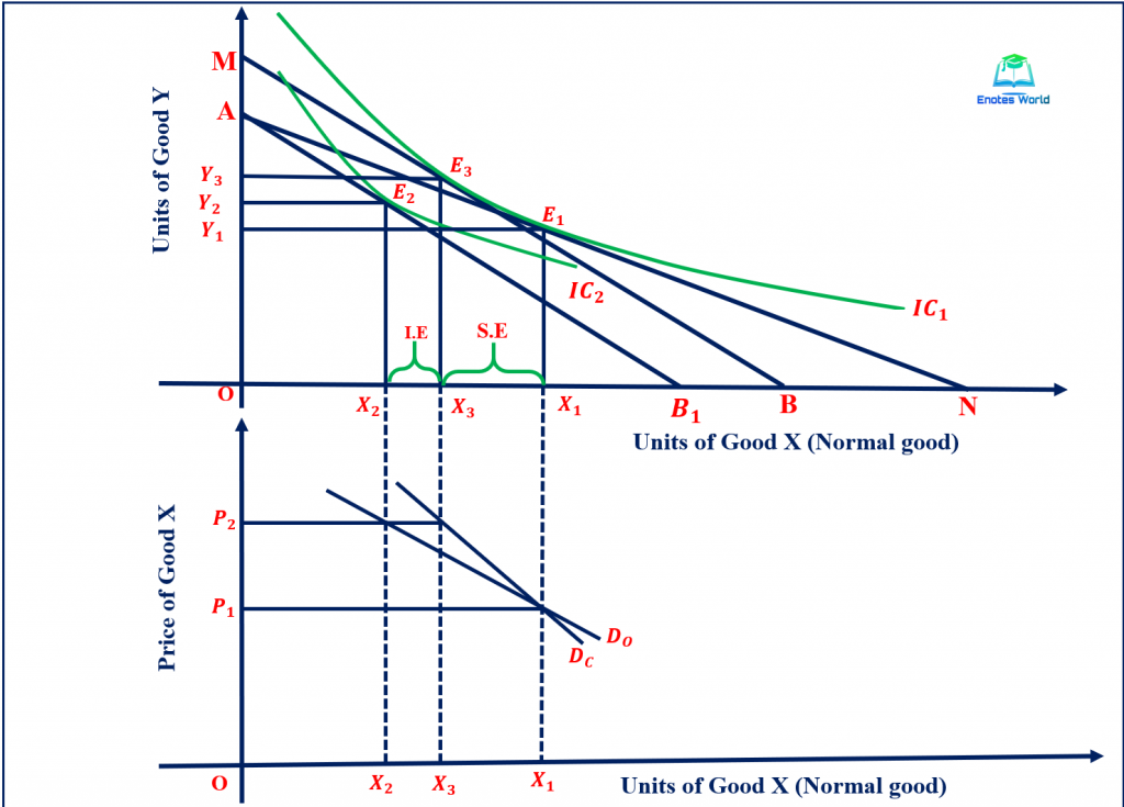
We assume there is a decrease in the price of the normal good (measured along with the x-axis), to derive the ordinary and compensated demand curves. The figure shows the derivation of such a demand curve in the case of a normal good and falls in the price of the goods measured in the x-axis.  

In the above figure, the upper part shows the comparative statics of consumer behavior with a fall in the price of good X. E₁ is the initial equilibrium on indifference curve IC₁ with optimum units of consumption of good X and Y as X₁ and Y₁ respectively. Suppose there is a decrease in the price of the good X. With a fall in the price of good X, there is an increase in the purchasing power of the consumer as represented by the rightward swing of the budget line from AB to AB₁. Due to an increase in the purchasing power of the consumer, now he or she can purchase more of X and the consumer is in the equilibrium at point E₂ on the higher indifference curve IC₂ with X₂ and Y₂ units of good X and good Y.

Here at point E₂ consumer has consumed the X₂ units of good X by reducing the Y₁Y₂ units of good Y. It has happened due to two reasons; one is that the commodity X has become cheaper relative to Y and consumer substitute cheaper good X for the dearer good Y; this is known as the substitution effect. Second, a fall in the price of good x increases the purchasing power of the consumer (increase in real income), and thus by using the available money income now the consumer can afford slightly more units of good X and Y both and known as income effect.

So, the movement from E₁ to E₂ has both income and substitution effects. The price decline has a positive substitution effect and for income effect, it is positive in the case of normal goods and negative in the case of inferior goods. 

Considering these two equilibrium points in the lower section of the diagram, we have got the points J and K showing two combinations of price and quantity demanded of good X. With initial price P1, the demand for good X is X1 and decrease in price from P1 to P2 increases the demand for good X from X1 to X2. By joining the points J and K, a downward sloping curve D_O is obtained. This curve is an uncompensated demand curve or ordinary/Marshallian demand curve.

Likewise, to derive the compensated or Hicksian demand curve, we have to keep real income constant. It means the increase in real purchasing power of the consumer as a result of fall in price is withdrawn by drawing an imaginary budget line MN, parallel to line AB₁ in such a way that it should tangent the initial indifference curve or lower indifference curve at point E₂, right to the initial equilibrium point E₁.

Thus, according to the idea of Hicks, money income should be decreased by the amount that would allow the consumer to keep himself or herself at the level of satisfaction he or she has derived from IC₁ before the change in price (real income constant). Now after the adjustment, the consumer is in equilibrium at point E₃ on the initial indifference curve and consumes X₃ units of good X and Y₃ units of good Y.

Here, the movement from the point E₁ to E₃ is the substitution effect, and the movement from E₂ to E₃ is the income effect. From the movement of the consumer’s equilibrium from point E₁ to E₃, the consumer has increased the consumption of good X by X₁X₃ units by reducing the consumption of good Y by Y₁Y₃ units. This is called the substitution effect of the decrease in price.

From the equilibrium E₁ and E_3, we got the two combinations of price and demand different than the combinations guided by the idea of Marshall. It is due to the adjustment of the real income of the consumer. The points J and L in the lower section of the point are obtained from the given equilibriums. By joining these two points derives a downward sloping demand curve D_C. This is the compensated demand curve for good X (normal good) when there is a fall in price. So, the compensated demand curve is derived, only considering the substitution effect of a fall in price.

Derivation of Ordinary and Compensated Demand Curve for the Rise in Price

Now here we assume there is an increase in the price of the normal good (measured along with the x-axis), to derive the ordinary and compensated demand curves. The figure shows the derivation of such a demand curve in the case of a normal good and a rise in the price of the goods measured in the x-axis.  

Let us consider the given initial information as; market price of good X is P_X, for good Y, P_Y, and the level of money income Y. With the given information, the consumer is in equilibrium at point E₁. It is the point where the initial budget line AB is tangent with the initial indifference curve IC₁ with X₁ units of good X and Y₁ units of good Y.

When the price of good X increases to P₂ from the initial price P₁ then the real purchasing power will decrease and the budget line will swing inside and budget line AB₁ will be the new budget line at which situation E₂ is the equilibrium point on the lower indifference curve IC₂ and lower demand for normal good X (X₂).  

To identify the substitution effect, we have to give the subsidy to the consumer in such a way that he would be able to equilibrium in the original indifference curve IC₁ at the point left to the original equilibrium E₁. The new budget line should be parallel to budget line AB₁. Here, the required budget line is MN and this line will tangent with the original indifference curve IC₁ at point E₃.

At the new equilibrium point after the adjustment, the demand for good X decreases from X₁ to X_3, and the demand for good Y increases from Y₁ to Y₃ leaving at the same level of satisfaction. Here, good X is a relatively expensive good, the consumer substitutes Y for good X. So, the movement from point E₁ to E₂ is the price effect, movement from E₁ to E₃ is the substitution effect, and movement from E₃ to E₂ is the income effect.

The demand curves keeping real income constant and money income constant are derived in the lower section of the diagram. The demand curve that keeps money income constant or alters the real income/ordinary demand curve can be derived with the help of equilibrium E₁ and E₃. These two equilibrium points give the combination of price and demand shown by points A and B in the lower part.

At point A, the price is P1 and demand is X1. With the rise in price and keeping money income constant (allowing alteration of real purchasing power doing nothing when the price falls), the real income will decrease and the consumer reduces the demand for good X from X1 to X2 represented by point B. By joining these points, A and B we derive the downward sloping ordinary demand of normal goods measured along with the x-axis at the situation of the rise in price.

Again, the demand curve keeping real income constant/purchasing power constant by altering the money income can be derived with the help of equilibrium points E₁ and E₃ in the lower part of the diagram. At equilibrium point E₁, the price of good X is P₁ with the demand of X₁ units. That has represented by point A. With the increase in the price of good X, the real income of the consumer is decreased, but we have to keep such real income or purchasing power constant as equal to the level equivalent before the change in price.

Thus, to do so the money income available to the consumer has to be changed/increased by the amount of AC or B₁D so the consumer can keep his or her level of satisfaction/real income constant as equivalent to the satisfaction obtained at point E₁. At this point after the adjustment, the consumer has reduced the consumption of good X from X₁ to X₃ with an increase in price from P₁ to P₂ as represented by point C in the lower portion of the diagram. Thus, by joining points A and C we get the downward sloping demand curve D_C and it is known as the compensated or Hicksian demand curve. 

Here, we only explained about change in prices rise and fall in the price of normal goods) and the derivation of the demand curve of normal goods. The derivation of demand curves with price changes in the case of inferior and Giffen goods will be explained in our further posts.