Introduction

A consumer attains his/her equilibrium when he/she maximizes his/her total utility, given his/her income and the prices of the two commodities. We combine the indifference curves and the budget line on the same diagram to illustrate the consumer’s equilibrium graphically. The indifference curve in the utility analysis assumes that the consumer tries to maximize his or her utility. Given the amount of money income that the consumer wants to spend on two commodities and given the price of two commodities, we can draw a budget line. While the budget line shows the various combinations that the consumer can afford to purchase with his or her given income or budget and given prices of two goods and the indifference map shows the consumer’s scale of preferences between various blends of two goods. Utility maximization subject to the budget constraint means getting to the highest possible indifference curve without going beyond the budget line. Here we explain the graphical as well as the mathematical illustration of the consumer’s equilibrium with the indifference curve approach.

For a detailed explanation and graphical derivation of the Consumer’s Equilibrium with the Indifference Curve Approach, click here.

Mathematical Derivation of the Consumer‘s Equilibrium

Suppose that a consumer consumes two commodities q₁ and q₂ with price p₁ and p₂ and money income M. Now we can mathematically derive the necessary and sufficient condition whereby he would maximize his utility.

Let the utility function U= f (q₁, q₂) and the budget line constraint be, M=p₁q₁+p₂q₂  

Where q₁= quantity consumption of commodity q₁ or the first commodity; q₂= quantity consumption of commodity q₂ or the second commodity; p₁= price of the first commodity or the commodity q₁; p₂= price of the second commodity or the commodity q₂; and M= money income.

A consumer is said to be in equilibrium when he or she maximizes utility under the budget constraint, then the statement of the problem can be expressed as;

Maximize U = f (q₁, q₂) ………… (i)

Subject to M= p₁q₁+p₂q₂…………. (ii)

Using the Lagrangian multiplier λ as,

V= f (q₁, q₂) + λ (M- p₁q₁-p₂q₂) ……. (iii)

Setting the first-order conditions,

V₁= ∂V/∂q₁=0

Or, ∂V/∂q₁=∂ [ f (q₁, q₂) + λ (M-p₁q₁-p₂q₂)] /∂q₁=0

Or, f₁– λp₁=0

Or, MU₁– λp₁=0

Or, MU₁=λp₁

Or, λ= MU₁/p₁…………. (iv)

Similarly,

V₂= ∂V/∂q₂=0

Or, ∂V/∂q₂=∂ [ f (q₁, q₂) + λ (M-p₁q₁-p₂q₂)] /∂q₂=0

Or, f₂– λp₂=0

Or, MU₂– λp₂=0

Or, MU₂=λp₂

Or, λ= MU₂/p₂…………. (v)

And,

V_λ=∂V/∂_λ=0

Or, ∂V/∂ _λ =∂ [ f (q₁, q₂) + λ (M-p₁q₁-p₂q₂)] /∂ _λ =0

Or, M-p₁q₁-p₂q₂=0………. (vi)

Now, differentiating equation (iii) with respect to M. we get,

∂V/∂M=∂ [ f (q₁, q₂) + λ (M-p₁q₁-p₂q₂)] /∂M= λ ∂M/∂M= λ

Or, ∂V/∂M=MU_m=λ…………. (vii)

Where MU₁= marginal utility of first (q₁) commodity; MU₂= marginal utility of second (q₂) commodity; and MU_m= marginal utility of money

If we combine equations (iv), (v), and (vii)

MU₁/p₁=MU₂/p₂ =λ= MU_m

Or, MU₁/p₁=MU₂/p₂ = MU_m………. (viii)

This is the condition for consumer equilibrium under the cardinal or Marshallian approach of utility analysis.

The First Order Condition Under the Indifference Curve Approach

The utility function U=f (q₁, q₂) and under the indifference curve the level of utility remains the same so, dU=0

Now, dU= d [f (q₁, q₂)]

Or, 0=∂ f (q₁, q₂) dq₁/∂q₁+∂ f (q₁, q₂) dq₂/∂q₂

Or, f₁ dq₁ + f₂ dq₂=0

Or, dq₂/dq₁=-f₁/f₂………… (ix)

The rate of change in q₂ w.r.to q₁ gives the slope of the indifference curve and it is negative.

Now, the marginal rate of substitution of q₂ for q₁ (MRS q₁, q₂) is also negative. We have to find the slope of the budget line M= p₁q₁+p₂q₂ by taking total differentiation.

Or, d M= d [p₁q₁+p₂q₂] (dM=0, budget is constraint)

Or, 0= p₁dq₁+p₂dq₂

Or, dq₂/dq₁=-p₁/p₂<0………. (x)

The slope of the budget line is also negative. Combining equation (ix) and (x) we get,

 dq₂/dq₁=- f₁/f₂=-p₁/p₂………. (xi)

This shows that the slope of IC= The slope of the budget line

So, from equation (xi),

f₁/f₂=p₁/p₂………. (xii)

The ratio of utilities is equal to the ratio of prices. So, the first order or necessary condition is that the ratio of marginal utility of two commodities must be equal to the ratio of their prices.

The Second Order Condition

Here, the second-order condition requires the strict convexity of the indifference curve at the point of tangency between IC and the budget line for the utility to be maximized. It means the slope or IC is decreasing but it must be positive. It can be obtained as;

d²q₂/dq₁2>0

Using the bordered Hessian determinant second-order condition requires that |H₂| <0 and |H₃|>0 

Here,

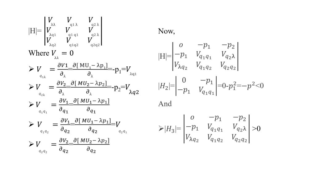
This implies that the indifference curve is strictly convex to the origin.

Therefore, the consumer can attain maximum satisfaction at that point where IC is tangent to the budget line as well as IC is strictly convex to the origin.