The key purpose of the analysis of consumer behavior is to derive a consumer demand curve. Here we will discuss the derivation of the demand curve under cardinal utility analysis in the case of one commodity and case of two commodities.

Learning Objective To deal with the derivation of the demand curve under cardinal utility analysis

Derivation from the Law of Diminishing Marginal Utility

To derive the demand curve based on the law of diminishing marginal utility, we measure the marginal utility of a commodity in terms of money as Marshall did. Measurement of marginal utility in terms of money means how much money a consumer is prepared to pay for a unit of the good.

The law of diminishing marginal utility says that as the quantity of a good with a consumer increases, the marginal utility of that good to him in terms of money diminishes. Thus, the marginal utility curve of good is downward sloping. According to the cardinal utility approach, a consumer reaches his equilibrium where MU_X=P_X in case of one commodity. This logic of consumer equilibrium in the case of a single good provides a fitting basis for the derivation of the individual demand curve for a commodity. Marshall has derived the demand curve from the consumer’s equilibrium for the first time under the condition of a single commodity. This equilibrium condition in a single commodity case is used to derive a demand curve.

As we know that the consumer is in equilibrium at the point where the marginal utility of a good is equal to its price. The downward-sloping marginal utility curve indicates that with a decrease in price the consumer will buy more of the goods so that its marginal utility also falls and becomes equal to the new price. So, the downward sloping marginal utility curve shows the downward sloping demand curve. It means the downhill marginal utility curve shows the fact that demand will increase with a fall in price. The following figure shows the entire process of derivation of the demand curve under cardinal utility analysis with a single commodity.

In the panel (I) of the above figure, the MU_X curve is diminishing the marginal utility curve of the good measured in terms of money. In panel (II) of the figure we measure price and quantity demand of good X. When the price of the good is P₁, the consumer is in equilibrium at point E₁ with the quantity demand of Q₁ because, at point E₁, MU₁ is equal to P₁.

Now assume price decreases to P₂ from P₁, the equality between marginal utility and the price is attained at point E₂. With the decrease in the price of the commodity, the consumer has to purchase more units of goods to reduce the marginal utility to make equality between reduced marginal utility and price. Thus at a decreased price consumer has purchased higher quantity and the marginal utility has also decreased and MU₂ becomes equal to P₂.

Again when price decreases to P₃, there is equality between lower marginal utility MU₃ at the higher quantity Q₃. Thus at price P₃, the consumer will demand Q₃ quantity of the good X. From this discussion we can infer that as the price decreases, the quantity demand increases, and marginal utility will decrease and the marginal utility will become equal to price. J, K, and L are the price-quantity blend equivalent to equilibrium E₁, E₂, and E₃ respectively. If we join the point J, K and L we well get the downward sloping demand curve. It is also known as the Marshallian demand curve.  

Derivation of Demand Curve from the Law of Equi-Marginal Utility

Here we will derive the demand curve with the help of the law of equi-marginal utility. It is the case in which consumer spends his limited income on several goods.

According to the law, the consumer is in equilibrium when the ratio of marginal utility and prices of each commodity are equal to the marginal utility of money. Therefore, the consumer is in equilibrium when he is buying the quantities of various goods (i.e. two goods) in such a way that satisfies the following rule:

MU_X/P_X=MU_Y/P_Y=MU_m(for two commodities case); and MU_X/P_X=MU_Y/P_Y=MU_n/P_n= MU_m(for n commodity case)        

And the budget constraint is,

P_XQ_X+P_YQ_Y=M (for two commodity case); and P_XQ_X+P_YQ_Y+……. + P_nQ_n=M (for n commodity case)

Where MU_m = marginal utility of money.

As mentioned previously, the equilibrium condition in two commodity cases is that per rupee marginal unit of each commodity is equated to the marginal utility of money. That is MU_X/P_X=MU_Y/P_Y=MU_m

Let us assume that the consumer has allocated his total income in consuming good X and Y and attending maximum satisfaction. Now suppose the price of good X falls whereas the price of Y and income of the consumer is constant and as a result, MU_X/P_X>MU_Y/P_Y=MU_m

To achieve equilibrium, the marginal utility of good X must be reduced which is possible by consuming more units of the commodity. So, it is clear that when the price of the commodity falls to attain the equilibrium condition, the consumer must consume more units of that particular commodity and vice versa. Therefore, the demand curve is downward sloping. The following figure helps to explain the derivation of the demand curve under cardinal utility analysis in the case of two goods.

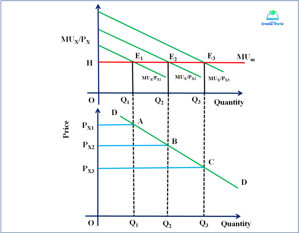
In the upper part of the figure, when the price of commodity X is P_X1, the equilibrium exists at point E₁ and where MU_X/P_X1=MU_m condition is fulfilled. In such a point the consumer is consuming the OQ₁ quantity of X.

Suppose when the price of commodity X is decreased to P_X2, then the MU curve shifted to MU_X/P_X2 from MU_X/P_X1. If the consumer consumed the same unit of commodity X at a reduced price then MU_X/P_X2 >MU_m and to get the equilibrium situation consumer should reduce the MU of X.

For this, he has to consume more units of X. So his consumption is OQ₂ and equilibrium E₂ has attained with MU_X/P_X2 =MU_m

Again, if the price reduces to P_X3 the MU shifted upward to MU_X/P_X3, and a new equilibrium existed at point E_3.

In the lower part of the diagram, the downward sloping demand curve shows the relation between price and demand. When there is price P_X1, the quantity demand is OQ₁. If the price decreases to P_X2, then the demand for commodity increased to OQ₂. And if price again reduced to P_X3 then quantity demand increases to OQ₃ and made a combination of point J, K, L and if we add all the points we get a downward-sloping demand curve in the case of two goods.

References and Suggested Readings

Ahuja, H.L.(1970). Advanced Economic Theory. Delhi: S Chand and Company Limited

Dwibedi, D.N. (2003). Microeconomics Theory and Applications. Delhi: Vikas Publishing House Pvt. Ltd.

Kanel, N.R. and et.al (2016). Microeconomics. Kathmandu: Buddha Publications

Mankiw, N.G. (2009). Principles of Microeconomics. New Delhi: Centage Learning India Private Limited