In our situation of good X, good Y, and money income M; if money income and the price of good Y stays the same but the price of good X rises, then the consumer will feel poorer, and if the price of good X falls, then the consumer will feel richer. This observation has led economists to try to separate the impact of a price change on quantity demanded into two components.  

1. The substitution effect: It involves the substitution of good X for good Y or vice-versa due to a change in the relative price of two goods.
2. The income effect: It involves the change in demand for the goods due to an increase or decrease in the consumer’s real income or purchasing power as a result of the price change.

The sum of these two effects is often called the total effect of a price change or simply price effect. The decomposition of the price effect into the substitution and income effect components (Income and Substitution Effects of a Price Change) can be done in several ways depending on what we would like to hold constant.

Methods of Decomposition of Price Effect into Substitution and Income Effect

There are two main methods of decomposition of total effects into substitution and income effect as suggested in the economic literature; first the Hicksian method and second the Slutsky method. Here we will discuss both of the methods of Income and Substitution Effects of a Price Change separately.   

The Hicksian Method of Income and Substitution Effects of a Price Change

For the detailed explanation of the decomposition of price effect into substitution and income effect under the Hicksian method please click here. 

The Slutsky Method of Income and Substitution Effects of a Price Change

A Soviet economist, Eugen Slutsky had proposed an alternative definition of the substitution effect, similar to the Hicksian substitution effect. In the Sulstky method, the increased income due to fall in price is adjusted or compensated so that the consumer can be on the original or the old indifference curve at the new set of prices. Thus, the Slutsky’s substitution effect is derived when the income adjustment is such that the consumer can buy the old bundle at the new set of prices. This method is also known as the cost difference method.

The following figure shows the process of decomposition of price effect into the substitution and income effect under the Slutsky method.

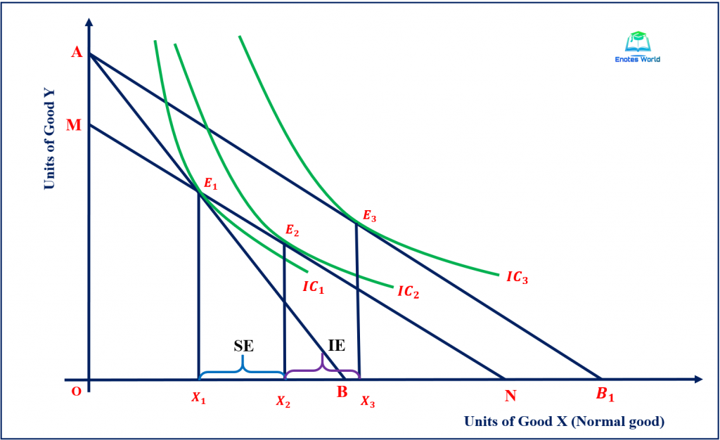
In the above figure, E₁ is the initial equilibrium with the consumption of X₁ units of good X and Y₁ units of good Y.  Let us suppose that the price of good X falls. This results in the outward rotation of the budget line from AB to AB₁. Due to the fall in the price of good X, the purchasing power of the consumer increases. To keep the purchasing power constant or the real income constant we draw an imaginary budget line MN through the original equilibrium point E₁ and parallel to newly rotated budget line AB₁.  

Drawing the new imaginary budget line through the original equilibrium point E₁ on the indifference curve IC₁ implies that his purchasing power remains constant and he or she can consume the original bundles if he likes.

When the consumer is in the original or initial purchasing power from the cutting down of increased purchasing power or real income due to a fall in the price of good X, the consumer compares the relative price of good X (the new decreased price of good X) with good Y. He or she finds good X relatively cheaper than good Y. The change in relative price results in the consumer to rearrange the purchase of good X and Y and as a result, the consumer will attend equilibrium at higher indifference curve IC₂ at point E₂. At point E₂, the consumer demands X₂ units of good X. Thus, here consumer substitutes X₁X₂ units of good X for good Y due to the lower price of good X (because of the relatively cheaper price of good X).

This movement from point E₁ to E₂ or from X₁ to X₂ is a substitution effect because it is the effect in consumption due to change in the relative price of the commodity X only, keeping the real purchasing power or real income constant.

If the increased real income has given back to the consumer then he or she will move to the new higher level of indifference curve with a higher level of satisfaction. It means the consumer’s equilibrium point moves from point E₂ to E₃ due to the increase in real income as a result of the fall in price. Thus, the consumer consumes X₃ units of good X and reaches a higher level of satisfaction. The movement from point E₂ to E₃ or, from X₂ to X₃ is the income effect.

Therefore, Total Price Effect (PE)= Substitution Effect (SE)+ Income Effect (IE)

Or, X₁X₃=X₁X₂+X₂X₃ or E₁E₃=E₁E₂+E₂E₃  

Comparison between the Hicksian Method and the Slutsky Method

The Hicksian method is theoretically the correct one, as with this method the substitution effect measures the effect of movement along an indifference curve due to change in relative prices, whereas the income effect measures the effect of a movement between indifference curves at unchanged relative prices. To find the substitution effect component of change in relative price, we use the compensating variation in the Hicksian method but we don’t know by how much amount of money income is reduced or withdrawn to keep real income constant. Thus, the equilibrium point (E₂ in our diagram of Hicksian decomposition) made by a newly drawn imaginary budget line on the initial indifference curve IC₂ is difficult to find in real life.

However, in the Slutsky method, we know the amount of money income that is to be reduced or withdrawn so that he or she would be able to get the same level of purchasing power after a fall in price. Here the newly shifted budget line passes through the initial equilibrium E₁ on the initial indifference curve IC₁ so that the consumer can purchase the initial bundle of goods even after the fall in price. Thus, the amount of money how much to reduce is known in this case.

For example, suppose that initially, the price of good X and Y are PX=Rs. 10 and PY= Rs. 10. The consumer’s income is Rs. 150. Suppose the consumer buys 7 units of X and 8 units of good Y. now PX falls to Rs. 5. Then in the Slutsky method, we take away Rs. 35 of the consumer’s incomes. With the income of Rs. 115 the consumer can still buy 7 units of X and 8 units of Y as before. The consumer will choose another bundle and this is what we have observed in our above graphical presentation. A similar realistic type of observation is not found in the case of Hicksain’s case, although we can talk theoretically about an income adjustment that will keep the consumer on the same level of the indifference curve. 

Although operational, the Slutsky method is not theoretically defensible, because the movement from original equilibrium (E₁) to upper equilibrium (E₂) involves a movement between indifference curves and thus is not a substitution effect. The method, in general, overestimates the substitution effect and underestimate the income effect. 

The following table shows the comparison between the above two methods of decomposition of the total effect on the income and substitution effect.

Hicksian Method	Slutsky Method
It is a compensating variation method	It is the cost difference method
The consumer remains on the same IC	Consumer moves on the higher IC
Change in money income is equal to compensating variation and it is unknown in terms of the amount	Change in money income is equal to cost difference and it is known.
A more convenient method to identify the substitution effect	It is easy to handle the income effect but a little difficult to deal with the substitution effect.
IE and SE cannot be known without the knowledge of the consumer IC map.	IE and SE can be obtained from directly observed fact.