Different factors directly affect the consumer’s equilibrium condition, including changes in the price of one good, the price of other goods, and money income. It means a change in the price of the goods; the price of other goods and the money income of the consumer brings a change in the consumer’s equilibrium from one point to another. In general, if the price falls, more of it is purchased, and vice versa. The overall change in quantity demanded due to a change in the price of the good, all the other things (income of the consumer and price of other goods) remaining the same is known as the total price effect.
So, the price effect is the change in the consumer’s equilibrium quantity of purchase as a result of the change in the price of goods only. With the change in the price of the goods and services, the consumer’s equilibrium point moves from one place to another and it is known as the total effect or total price effect. Here we will explain the meaning of the substitution effect and the decomposition of the price effect into substitution and income effects.
Contents
Meaning of Substitution Effect (SE)
The substitution effect is the change in quantity demanded of a commodity due to a change in its relative price alone, with the real income of the consumer remaining the same. It means SE is the change in quantity demanded of a commodity due to a change in the relative price of the same commodity keeping the real income and price of other goods constant. Therefore, SE relates to the change in the quantity demand resulting from a change in the relative price of the goods
For example, SE relates to the increase in the quantity demand of good X when its price falls while keeping the real income and price of Y remain constant. In such cases the consumer substitutes cheaper goods X for the relatively dearer goods Y. When there is a fall in the price of good X, the real income of the consumer will increase but an increase in real income of the consumer is maintained constant to see the substitution effect.
According to Dominick Salvatore, the substitution effect measures the increase in the quantity demanded of a good when its price falls resulting only from the relative price decline and independent of the change in real income.
In the words of A. Koutsoyannis, the substitution effect is the increase in quantity bought as the price of the commodity falls, after adjusting income to keep the real purchasing power of the consumer the same as before.
When there is a change in the price of a commodity then there is a change in demand. Here demand changes due to two reasons as;
- One is that the commodity now becomes relatively cheaper or expensive/dearer and demand will be affected
- Second is that when there is a change in price then the purchasing power also changes and as a result there is a change in demand
And now suppose the price has declined then;
The commodity will become cheaper and the consumer will buy more of it by substituting cheaper for dearer/expensive. It is called the substitution effect. Likewise, with a fall in price, there is an increase in real income or purchasing power so demand will be increased. It is called the income effect.
Therefore, Total Price Effect=Substitution Effect + Income Effect
Therefore, the substitution effect is the change in demand for a commodity due to a change in its relative price only, keeping the real purchasing power constant.
Income Effect (IE)
The income effect is the change in the quantity demanded of a commodity because the change in its price has the effect of changing a consumer’s real income. The decrease in the price of the commodity will increase the purchasing power of consumer or the real income of the consumer, and as a result, if there is an increase in demand for a commodity then it is known as the income effect.
Graphical Presentation of the Substitution Effect
Suppose, there are two substitute goods X and Y. When there is a decrease in the price of a good, X then the consumer’s real income increases. Now the buyer can purchase more quantity of good X. Here the buyer can buy more not because his/her money income has increased but due to the price of X has dropped. Thus, the rise in the consumer’s real income as a result of a fall in the price of commodity X has to be compensated to cancel out the gain in his or her real income. The compensation places the consumer at the same level of satisfaction as he/she was before. This is identified as the substitution effect.
The following figure helps to describe the concept of the substitution effect.
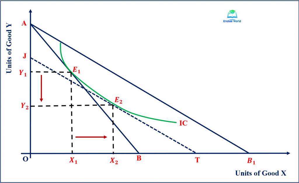
In the above figure, units of good X and Y are presented along the x-axis and y-axis respectively. AB is the initial budget line and it is tangent with the indifference curve IC at point E1. So, E1 is the initial equilibrium point. At the initial equilibrium point E1, the consumer purchases X1 units of good X and Y1 units of good Y.
Now, suppose that the price of good X decreases, then the real income of the consumer or purchasing power of the consumer increases. With an increase in real income, the initial budget line swings outward to AB1. To find the substitution effect, the increase in the real income of the consumer as a result of the fall in the price of good X should be adjusted so that the consumer stays on the same level of satisfaction/same indifference curve. Now to withdraw the increased real income, a hypothetical budget line JT parallel to the budget line AB1 is drawn. The budget line JT is tangent to the indifference curve at point E2. This parallel line JT is called the compensated budget line or a compensated variation and use to adjust income to keep the real income of the consumer the same as before, i.e., at the same indifference curve.
The movement from the equilibrium point E1 to E2 of the same indifference curve is the substitution effect. At a new equilibrium point E2, the consumer buys more quantity of good X by X1X2 units by reducing the units of good Y by Y1Y2 and remains at the same level of satisfaction (at the same indifference curve). It shows that the consumer is neither better off nor worse off than before. In the figure, we see that the consumer has substituted good X for good Y as good X has become relatively cheaper due to a decrease in its price and good Y remains dearer and the consumer attains the same level of pleasure.
Decomposition of Price Effect into Substitution and Income Effects
Graphically the decomposition of the price effect into substitution and income effects is done using the indifference curve with the budget line of the consumer. There are two approaches to separating the total effect into income and substitution effect namely the Hicksian approach and the Slutsky approach. Here we will discuss the Hicksian approach of decomposition of price effect into substitution and income effects.
We exemplify the decomposition of the price effect into substitution and income effects with the help of the following graph.
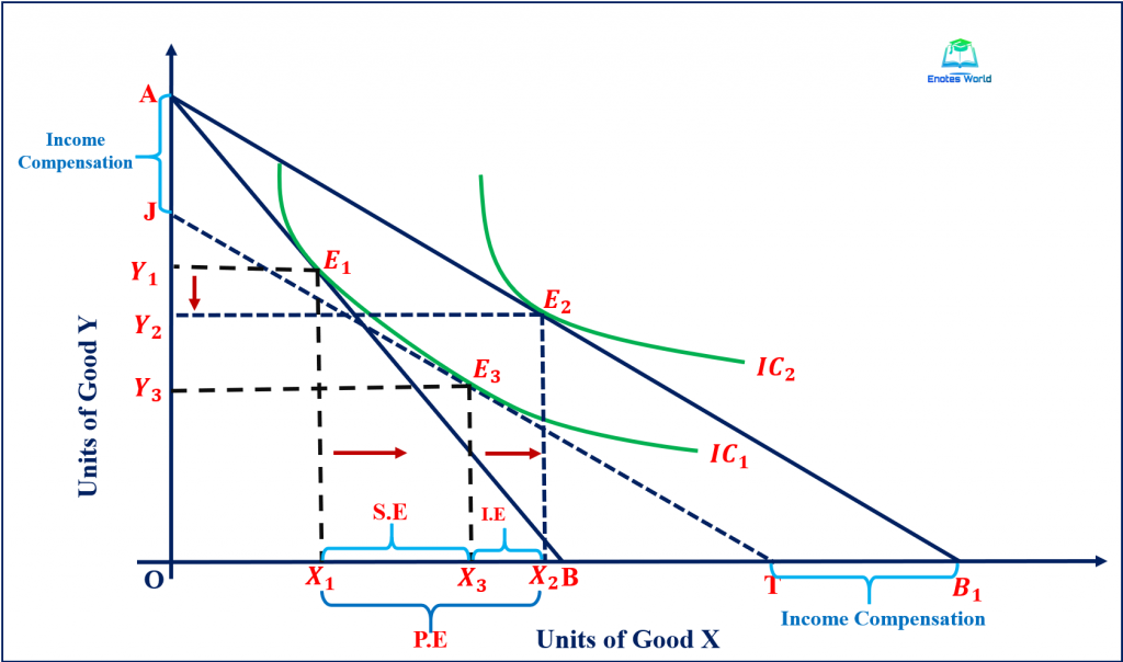
In the graph, the x-axis represents units of good X and the y-axis represents units of good Y. AB is the initial line tangent with indifference curve IC1 at point E1 with X1 units of good X and Y1 units of good Y. Suppose that there is a decrease in the price of good X and as a result, there is an increase in the real income of the consumer represented by the rightward swing of the budget line from AB to AB1. With the budget line AB1, the consumer attains equilibrium at the tangent point of the budget line and higher indifference curve IC2 at point E2. At the equilibrium point E2, the consumer can purchase X2 units of good X and Y2 units of good Y.
Here the movement from equilibrium point E1 to E2 is known as the total price effect or the price effect. As we know, this price effect consists of income and substitution effects. Now to the decomposition of the price effect into substitution and income effects, we require the withdrawal of increased real income of the consumer resulting from the fall in the price of good X.
Thus, to separate the total effect (Movement from point E1 to E2) the consumer’s increased real income or increased purchasing power is to be compensated by reducing the money income through the way of taxation according to Hicks, and so that the real income of the consumer becomes the same as before. This adjustment in income is known as compensating variation that is shown graphically by a parallel shift of new budget line AB1 until it becomes tangent to the initial indifference curve IC1 at point E3. This is shown by line JT. The reason for the compensating variation in income is to allow the consumer to remain on the same level of satisfaction as before the price change. Thus, line JT is known as the compensated budget line.
Now the movement from point E1 to E3 on the same indifference curve (IC1) shows the substitution effect of the price change. Here, the consumer buys more units of good X because it has become relatively cheaper than before, and thus he substitutes expensive or dearer good Y for good X. So, moving from point E1 to E3 increases the units of good X by X1X3 and reduces the units of good Y by Y1Y3, and the consumers remain at the same level of satisfaction.
Again, if the withdrawn or reduced money income of the consumer is given back or if the consumer is allowed to use his increased purchasing power, the consumer would move to point E2 on the upper indifference curve IC2 from point E3. In this case, he will use a part of his increased real income on the purchase of good X, and move from X3 to X2 or move from E3 to E2. This shift from E3 to E2 is known as the income effect. The compensated income in terms of good X is TB1 and in terms of good Y is JA which is known as compensating variation in income in the Hicksian approach. The entire effect can be written as;
Movement from E1 to E2 or X1 to X2 = Price Effect (PE)
Movement from E1 to E3 or X1 to X3= Substitution Effect (SE)
Movement from E3 to E2 or X3 to X2= Income Effect (IE)
From the figure, we can say that;
X1X2=X1X3+X3X2 Or, PE=SE+IE
Conclusion
The price effect is the totality of income and substitution effect. It means that the total price effect can be split into two components as income effect and substitution effect. According to the Hisksian substitution effect, when the price of any good falls (say good X) money income of the consumer is reduced by the amount of real income increased so that real income becomes constant implying that the consumer is neither better off nor worse off than before.
In the case of a normal good, the substitution effect is negative as to maintain the same level of satisfaction on the same indifference curve, a consumer increases the quantity demand of goods X whose price has fallen, and decreased the quantity demand for good Y as the price of X becomes relatively cheaper than the price of Y. The income effect is positive. Thus, the decomposition of the price effect into substitution and income effect can be done with the help of the indifference curve and budget line.
References and Suggesting Readings
Acharya, K.R. (2018). Microeconomics. Kathmandu: Asmita Books Publishers & Distributors (P) LTD.
Ahuja, H.L. (2017). Advance Economic Theory. New Delhi: S. Chand & Company.
Dhakal, R. (2019). Microeconomics for Business. Kathmandu: Samjahan Publication Pvt. Ltd.
Kanel, N.R. and et. al. (2019). Microeconomics for Business. Kathmandu: Buddha Publications.