Background and Concept of Preference Ordering
| Learning Objective To explain the concept of preference ordering and axioms of preference ordering |
Every individual consumer or each household has a fairly accurate notion of money income for a reasonable period. It also has some notion (perhaps not well defined) of the goods and services it wants to have. The task confronting every household is to spend its limited money income to maximize its economic well-being. No household or individual succeeds in this task. To some extent, this failure is attributable to the lack of accurate information including other reasons such as impulse buying. The consumer always gives his or her conscious effort to attain maximum satisfaction from a limited money income. Here we explain the preference of the consumers/preference ordering and its related axioms.
Every consumer is king in his or her choices based on the availability of economic resources. In economics, everything that provides satisfaction or holds want satisfying capacity is goods or services, or commodities. So, the scope of commodities is wider. The consumer can choose any of the commodities or the bundle of the commodity affected by many factors like income, the place where he or she lives, the allocation of his or her time between work and leisure, and so many other dimensions of consumer behavior. Considering the possible effect of all the control variables, every consumer selects the possible best combination of goods or bundle of goods among the available alternatives based on their relative want satisfying capacity so as to ensure maximum satisfaction. This is simply known as preference ordering or preference.
The analysis of such behavior of the consumer is greatly affected by the use of a utility function that assigns a numerical value or utility level to the bundles of commodities. In practical life, we may find it difficult to accept as the idea is a highly subjective phenomenon of consumer preference and depends on each buyer’s psychological aspect. If the consumer prefers to bundle A over bundle B, the utility function has to assign a larger numerical value to bundle A than to bundle B, but the actual numerical values so assigned are irrelevant. Similarly, if the consumer is indifferent between bundles A and B, the utility function must assign the same numerical value to each bundle, but the particular value so assigned is irrelevant. Assigning the numerical values to obtain satisfaction or utility is the interest of the cardinal utility analysis approach.
The measure of consumer preference or preference ordering can be done through the graphical model as well known as ordinal utility analysis. The graphical representation of consumers’ preferences is done by a graph called the indifference curve. But the consumers are constrained in making their choice due to the limited amount of income. This is represented by the budget constraint or price/budget line of the consumer. Combining the indifference curve and the budget constraint, we can define the consumer’s optimal choice from his or her preference ordering or preference ranking.
Whatever the way of analysis, the objective of the consumer is identical and it is to maximize the utility function subject to budget constraints. Here utility function is nothing more than an algebraic description of consumer preferences.
Let us consider a consumption bundle as denoted by a vector;
Xi= (X1, X2…. ,Xn).
Where Xi, i= 1, 2…, n, is the ith good in the bundle, and each Xi is non-negative. It means a consumer can have either zero or positive units, which is perfectly divisible. Here the term perfectly divisible means a consumer can buy or consume any amount or quantity of goods in a bundle. For instance, if there is 5kg of the quantity of one commodity in the bundle and a consumer can demand or consume 1 kg or 0.5 kg of that commodity according to his or her preference. It is called perfectly divisible. The preference of the consumer is a non-negative phenomenon. It means any consumer can not consume less than zero units of the commodity, therefore, if the person is not consuming any goods then his consumption is zero, no negative.
Thus, a consumer can rank the consumption bundles in the feasible set according to preference ordering and choose the one which is highest in the ranking or order. So, the preference ranking or preference ordering holds certain assumptions to make the study more systematic and accurate.
For example,
XI>XII means XI is preferred to XII that is XI is better than XII.
XI~XII means XI is indifferent to XII which is XI and XII are equally preferable.
XI≥XII means XI is preferent indifferent to XII that is XI is better than XII or XI and XII are equally preferable or both.
Assumptions/Properties/Axioms of Preference Order
The assumptions or the desired properties of the consumer’s preference ordering are briefly explained below;
Completeness Property: For any pair of bundles x and y, either x ≥ y or y ≥ x or x ~ y is possible to make.
It means that the completeness of the consumer’s preference implies that out of any two goods say A and B, the consumer either prefer A to B or B to A or becomes indifferent between A and B. This ensures that there are no ‘holes’ in the preference ordering of the consumer. Thus, the consumer is always in a position under which his decision will surely come. He or she can not say he or she does not know otherwise the best-preferred bundle is not known. The consumer is always in either position among given cases and this is called completeness.
Transitivity Property: For any three bundles of goods x, y, and z, if x ≥y and y ≥ z then x ≥ z.
It means the consumer’s preference is transitive. This assumption ensures consistency in consumers’ choices. For example, if a consumer prefers a car over a bike and a bike over a cycle then according to the transitivity axiom car would be preferable over the cycle. If the consumer here prefers a cycle over a car then the choice is not considered the consistent choice and would be known as non-transitivity. The same process is applied to the indifferent situation of the consumer for the given bundle. It means if the consumer is indifferent between Apple iPhone and Samsung and between Samsung and Xiaomi then he will also be indifferent between Apple iPhone and Xiaomi. So, the consumer can rank all the available bundles in the market in a consistent manner.
Reflexivity Property: Any bundle x is always at least as preferred as itself; i.e. any bundle is at least as good as an identical bundle (x ≥ x)
It means any bundle is preferred or indifferent to itself. This assumption seems unimportantly true. It ensures that every bundle belongs to at least one indifference set, namely that containing itself if nothing else. It is the plausible assumption for all most adult behavior but occasionally the behavior of small children may violate this assumption.
Non-Satiation Property: A consumption bundle x will be preferred to y if x contains more of at least one good and no less than any other, i.e. if x > y.
It means that the consumer always prefers a commodity to less. The bundle having more commodities will be preferred in preference order to maximize satisfaction. Moreover, this holds however large the amounts of goods in the bundle, hence the term non-satiation applies, and thus the consumer is never to be satisfied with the goods. Thus, for every consumer more is better. The following figure helps to get this axiom more clearly.
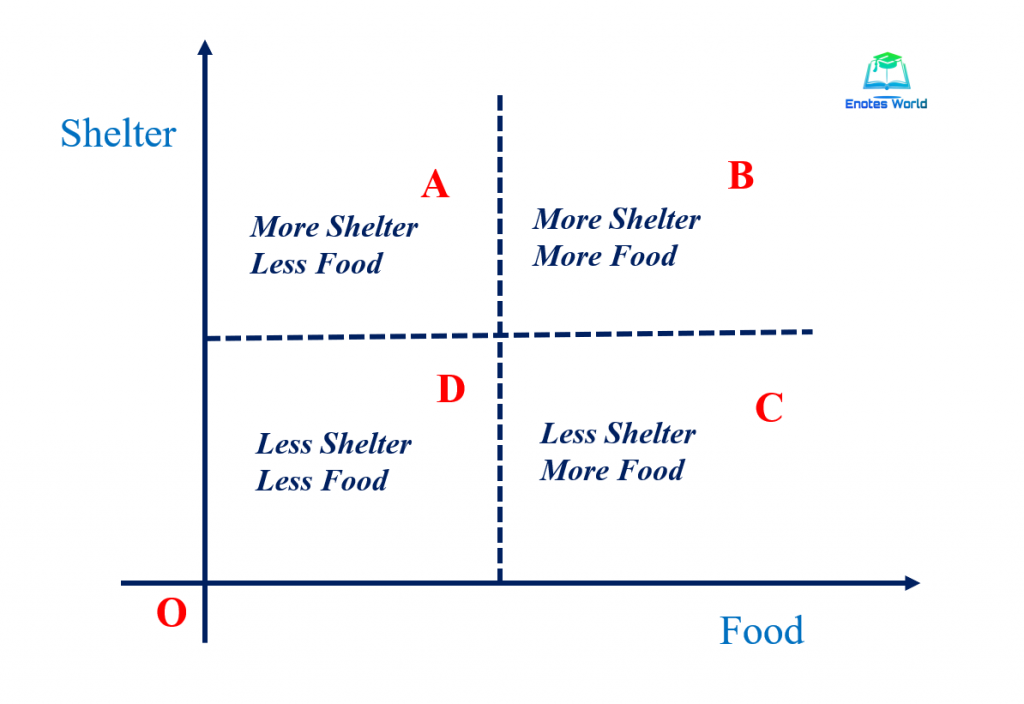
In the above figure bundle, B has more food and more shelter and is preferred over all the bundles. It is because, in bundle A, one is more and another is less and the same is in bundle C also. In bundle D, both are in fewer amounts. Thus, this assumption means that if a consumer has offered at least two bundles having the same commodities and one of those has more of both than is preferred. Thus, has been found in bundle B in our diagram. Regarding bundles A and C in the figure, we can not say anything, and only based on the principle of non-satiation bundle B is preferred in the preference ordering of the consumer.
Continuity Property: The graph of an indifference set is a continuous surface
It means the consumer’s preference is continued in the sense that there are no jumps and irregularities in the choices. In terms of consumer’s choice behavior, given two goods in his consumption bundle, we can reduce the amount he has of one good, and however small this reduction is, we can always find an increase in the other good which will exactly compensate him, leave in the same level of satisfaction.
Strict Convexity Property: Given any consumption bundle x, its better set is strictly convex.
It means the preference or utility function of the consumer is convex to the origin. The diminishing marginal rate of substitution between the commodities ensures the strict convexity of the utility function. The curvature shape of the indifference curve ensures the strict convexity of the utility function. The following figure helps to understand the significance of strict convexity axioms in utility analysis under the ordinal utility approach.
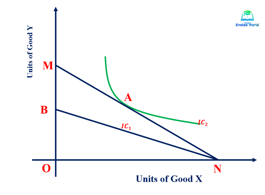
The term strict convexity in consumer theory implies that the second derivative of the utility function is diminishing but positive. That is ∆2Y/∆X2=d2Y/dX2>0. If the slope is equal to zero then that implies that the line can be straight or linear and there is no slope associated with it. So, the line with strict convexity recurs with the strict has to have a slope. In the above figure, IC2 is strictly convex, and the budget line MN and IC1 are simply convex or linear but not strictly convex. In terms of utility theory, there is a point of tangency between the budget line and the indifference curve, and the indifference curve is considered to present a well-behaving preference due to or in the form of its strict convexity.
Point A in the above figure shows such a point. At that point, the strictly convex curve is tangent to the linear budget line. If we see the indifference curve IC1 it isn’t strictly convex and can be linear. The linear IC only touches the linear budget line at point N but they are not tangent to each other and they don’t share the same slope as IC2 and budget line MN do at point A. Moreover, the linear IC shows that the consumer can consume only one good as well as that is not the interior solution. An interior solution occurs when both goods are consumed. Thus, the diminishing MRS X and Y at point A ensures the strict convexity axioms of preference ordering.
References and Suggested Readings
Ahuja, H.L. (2017). Advance Economic Theory. New Delhi: S. Chand & Company.
Gravell, H. and R. Rees. (2004). Microeconomics. Pearson
Koutsoyiannis, A. (1991). Modern Microeconomics. Hongkong: ELBS