Learning Objective To explain the technique and solution of the consumption decision problem

Once the consumer identifies his or her preference concerning several consumption bundles represented by the indifference map and which bundles can or cannot be afforded represented by the budget line, the decision problem is now related to the consumption decision. The straightforward answer is that the consumer will prefer only those bundles that can be afforded and that can maximize the satisfaction or utility function. It means based on the ranking of the consumption bundles as well as the feasible set of consumption bundles, the consumer takes consumption decisions, given the money income and prices of the goods. Here the consumption decision of the consumer is guided of affected by the axioms of preference ranking. Thus, the process of finding the optimal consumption bundle, given the feasible set of preferences, assumptions, and axioms, limited money income, and prices of the goods in the bundles is known as the consumption decision.

Regarding the arrival at the optimum consumption decision, we may express preferences mathematically in the form of the utility function. The utility function refers to the mathematical function that assigns a particular number to any consumption bundle and that helps to represent the preferences in a particular rank. Here the assigned mathematical values have no meaning in the sense that they are assigned only to show the preference ranking or preference ordering. Thus, here all is happening to maximize the objective function or to see the optimum level of pleasure subject to the money income. The objective function is nothing, but the utility function that is mathematically representing the preference of the consumer.

Based on the above discussion the objective function and its constraint can be expressed as;

Max. U (x₁, x₂, …., x_n)  

Subject to P_X. Q_X+P_Y.Q_Y+…. P_n.Q_n ≤ M or, S_t p_ix_i ≤ M,  x_i≥0, i=1,…,n.

The solution to our utility problems will be discussed in our coming discussions. Here we will derive the solution to the consumption problem of the problem with the help of the graphical representation. The following figure helps to show the consumption decision of the consumer.  

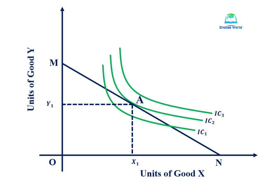
In the above figure, IC₁, IC_2, and IC₃ are three different indifference curves representing consumer’s preferences with different levels of utility. We can put several indifference curves in the graph (indifference map). There is a tangency solution where the optimal bundle A is such that the highest attainable indifference curve IC₂ is tangent to the budget line and the consumer consumes certain units of both the goods. The slope of the IC is equal to the slope of the budget line at the optimal point A.

d_y/d_x/ _{u constant} = d_y/d_x/ _{M constant}

Here, the initial expression shows the slope of IC and later shows the slope of the price line. We know that the slope of IC, as well as the slope of the price line, is negative. Here we are taking the absolute value of the slopes for the analysis purpose (Negative of the slope of the IC is MRS, and the negative of the slope of price line is the ratio of prices of x and y). Thus, the consumer’s optimal consumption decision requires;

MRS _x, _y = u_x/u_y=p_x/p_y

So, the consumer is in equilibrium or choosing an optimal bundle of goods when the rate at which he can substitute good for another on the market exactly equals the rate at which he is just happy to substitute one good for another.

Suppose the consumer spends one extra unit of money on good x, he would be able to buy 1/p_x units of good x. So, u_x.∆x is the gain in utility from an additional ∆x unit of good x. Hence, u_x/p_x is the gain in the form of utility from spending an additional unit of money on good x. u_y/p_y has also the parallel interpretation. The consumer will therefore be maximizing utility when he allocates his income between x and y so that the marginal utility of expenditure on x is equal to the marginal utility of expenditure on y;

u_x/p_x=u_y/p_y

Suppose the consumer’s income increases by a small amount.  Now he is indifferent between spending on x and y and thus utility would rise by u_x/p_x=u_y/p_y. Thus, the increase in consumer’s utility due to the increase in income is termed as the marginal utility of money u_m then we have;

u_x/p_x=u_y/p_y= u_m

The Corner Solution of the Consumption Decision

It is the case; the indifference curve touches the budget line and either of the axis. The following figure helps to explain the corner solution.

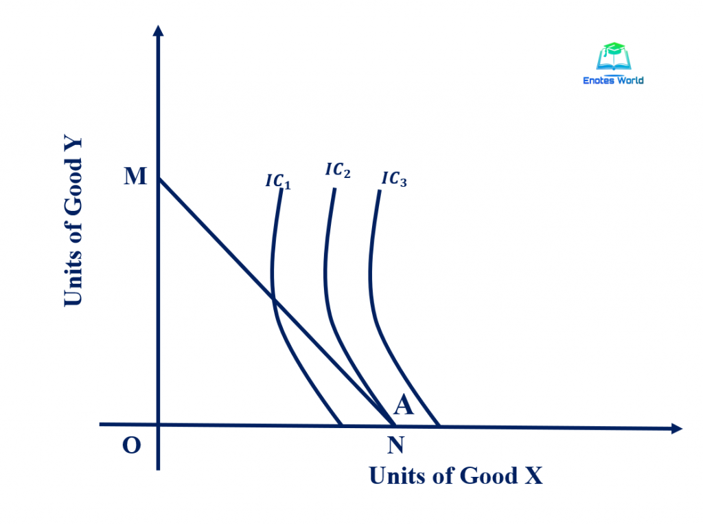
The above figure shows the case of the corner solution relating to the consumption decision. In the figure, the optimal solution point A does not shows any quantity of good ‘y’.  So, the budget line MN is less steep than the indifference curve i.e. the slope of IC is greater than the slope of the price line.    

d_y/d_x/ _{u constant} > d_y/d_x/ _{M constant} and MRS _x, _y = u_x/u_y>p_x/p_y

Rearranging the condition,

u_m= u_x/p_x>u_y/p_y

It shows that the marginal utility of expenditure on the good x is higher than the marginal utility if expenditure on good ‘y’, the good ‘y’ is not purchased. Due to the higher marginal utility of expenditure on good x than on y good, the consumer would like to move further down the budget line substituting x for y but is controlled by the fact that consumption of the negative amount of y is not possible.  This is how we can find the corner solution relating to the consumption decision of the consumer.   

References and Suggested Readings

Ahuja, H.L. (2017). Advance Economic Theory. New Delhi: S. Chand & Company.   

Gravelle, H. and R. Rees (2004). Microeconomics. Third edition, Pearson.