In this article, we have explained the static and dynamic analysis of macroeconomics.

Introduction to Static and Dynamic Analysis of Macroeconomics

To construct the economic model, there are two methods static and dynamic.  An economic analysis that limits its attention to the final equilibrium position is called ‘statics’ or ‘static’. A static model may be simple and comprehensive and irrespective of its type, it merely strengthens on the equilibrium spot. On the other hand, ‘dynamic’ analysis deals with the time it takes for an equilibrium position to be achieved after it is broken down. Thus, dynamic analysis is related to the overall path by which variables approach their equilibrium states.

Dynamic analysis also can be described as the study of the movement of economic variables from one equilibrium position to another. It retains a tie to the equilibrium notion but is concerned fundamentally with the state of disequilibrium and with adjustments or changes. Therefore, considering the time elements, the association between different macroeconomic variables (macroeconomics analysis) can be separated into three types.

Macro Static

Macro static is concerned with the study of the relationship between different macroeconomic variables such as total consumption, total income, and total investment in the state of equilibrium representing a particular point in time. The major features are:

• The nature of equilibrium is static, and it ignores the passage of time and therefore cannot explain the process of change in the model.
• Macro-static assumes there is no disturbance in the equilibrium position of the economy, and it believes it remains stable or stationary.
• It does not study the process to show how the economy has reached there or how the process of adjustment takes place.
• It only sees the final position of equilibrium of an economy and shows the still picture of the economic system.

For example, the position of the final equilibrium can be explained by using the Keynesian model of income determination. The equational form of the Keynesian income determination model in the state of equilibrium is Y=C+I; Where Y= National income/output, C=Total consumption expenditure, and I= Total investment expenditure.

This expression describes the association between three macroeconomic variables, Y, C, and I. Y=C+I signifies the static equilibrium as all the variables are belonging to a particular point of time and the system is in the state of equilibrium as Y is aggregate supply and C+I is aggregate demand.  It can be further explained with the help of the given diagram.

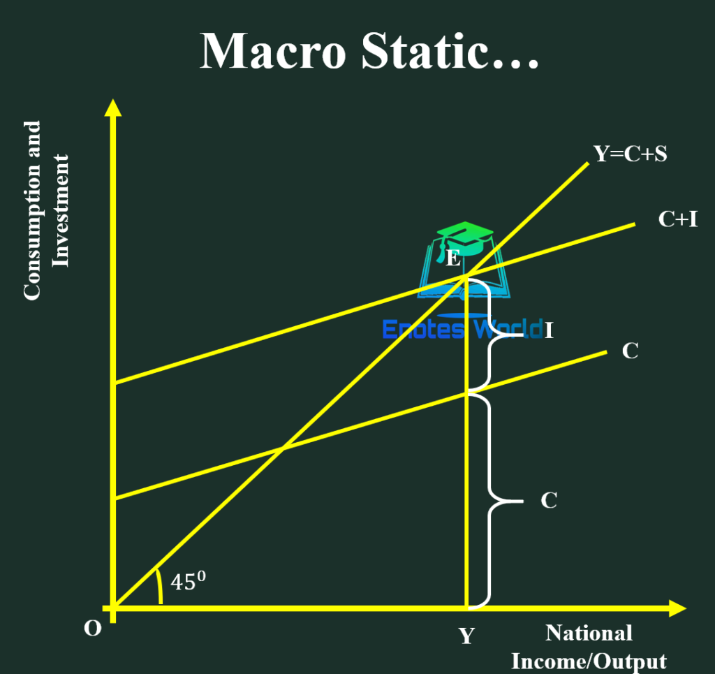
In the figure, the 45-degree line represents the aggregate supply function and the C+I line represents the aggregate demand line or function.  At point E, aggregate demand and aggregate supply lines are intersected with each other and determine the OY level of national income.

This shows the equilibrium value of macroeconomic variables at a given point in time and thus this is a static macroeconomic relation.

Comparative Macro Static

Comparative macro static is an analysis of change in equilibrium from one position to another. So, it compares the equilibrium positions of macro variables at different points in time. Macro variables in an economy are subject to change over time and such changes disturb the equilibrium position in an economy.

After a certain time, lag, a new equilibrium is established once again. Thus, comparative macro statics is concerned with a comparative study of such equilibriums-the original equilibrium to the new equilibrium.  However, it does not study the whole process of adjustment by which the economy shifts from one equilibrium position to another equilibrium position.  In comparative macroeconomics, we compare two static macro equilibriums or two different equilibrium positions representing two different points in time.

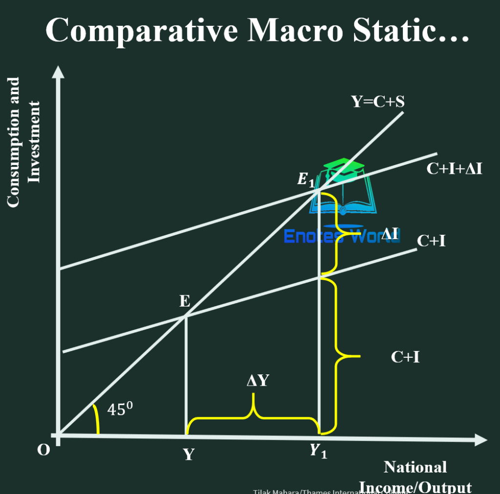
As shown in the figure, the economy is initially in equilibrium at point E, where the AD and AS curves together determine the equilibrium level of national income as Y.

Now suppose there is an increase in autonomous investment by ΔI amount. As a result, the AD curve shifts to C+I+ΔI, where it intersects the AS curve at point 𝑬_𝟏 with the equilibrium level of income 𝒀_𝟏. Here, comparative macro static compares equilibrium position E and 𝑬_𝟏 and it does not explain the actual process that the system follows over time to reach the new equilibrium point 𝑬_𝟏.

Macro Dynamics

Dynamic is a system of movements that is never in equilibrium. The macrodynamic analysis deals with the time and path that the system takes and follows to establish a new equilibrium after it is broken down due to changes in different macroeconomic variables. So, macro-dynamics studies the process through which a new equilibrium is established after a change in an independent economic variable. The major features of macro dynamic analysis are listed below.

• It describes the time and path taken by macroeconomic variables to move from the old equilibrium position to the new equilibrium position
• Economic dynamics is the study of the economic phenomenon in relation to preceding and succeeding events
• It illustrates the reasons for the breakdown and reestablishment of macroeconomic equilibrium
• It takes a realistic approach by assuming all the economic variables as changeable
• It describes all the happenings and phases of disequilibrium between initial and new points of equilibrium

Macro dynamic analysis can be explained with the help of the following diagram.

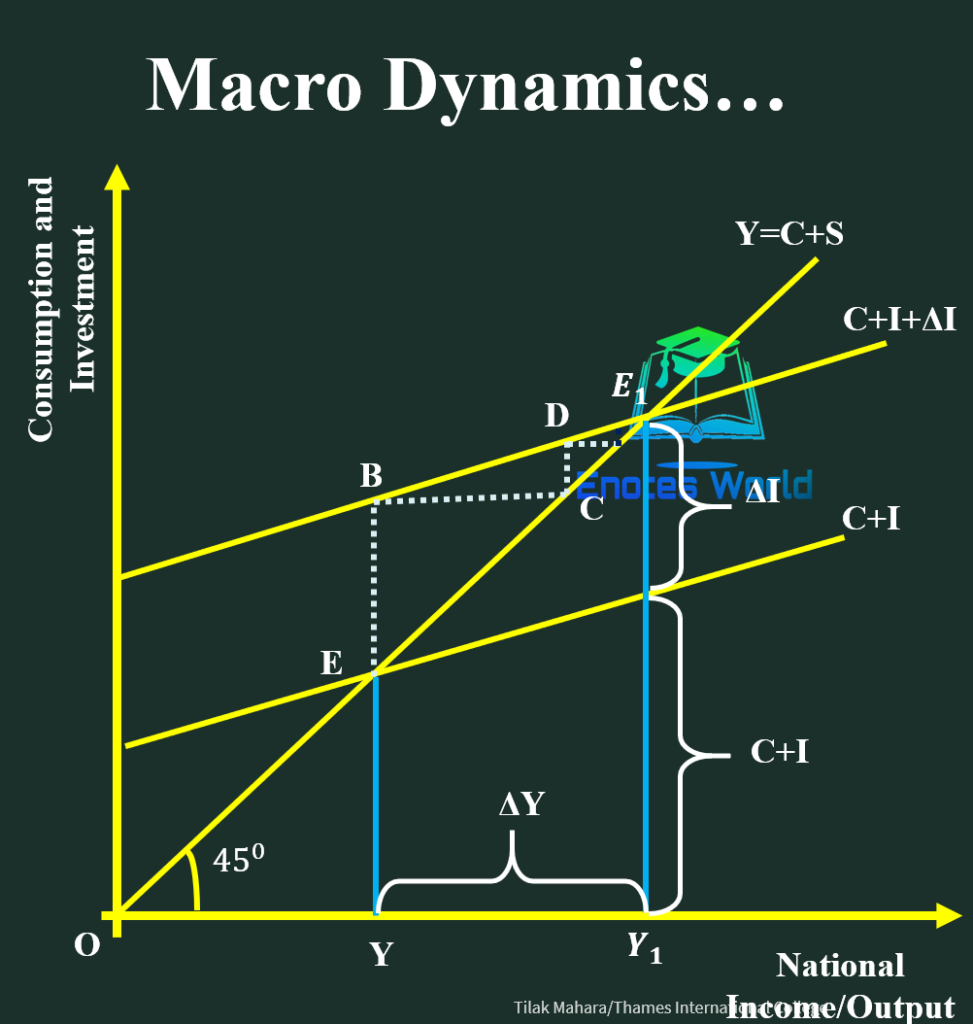
The economy is initially in equilibrium at point E where AD and AS curves are equal, and the OY level of equilibrium national income is measured. Suppose there is an increase in autonomous investment by ΔI amount. This causes a shift in the AD curve to C+I+ ΔI which intersects with AS curve at point 𝑬_𝟏.

The new equilibrium is formed due to a rise in investment expenditure. This new equilibrium is obtained after following the path that the variables approached over time

The actual path followed between equilibrium positions is shown by points B, C, and D. These points show a disequilibrium situation. The overall explanation of this path of establishment of equilibrium is analyzed by dynamic study.