Contents
Introduction
The laws of returns to scale explain the input-output relationship under the condition that both the inputs (labor and capital) are variable and their quantity increases proportionately (by same size or proportion) and simultaneously. When both the inputs labor and capital are increased proportionately, the scale or volume of production also increases. So, the law showing the input-output relationship under the condition of increasing scale of production is known as the law of returns to scale.
The Laws of Returns to Scale explains the behavior of long-run production function. In the long run, the supply of all the factors of production like land, labor, capital, etc. can be changed or supply is elastic as there is enough time for the producer to adjust the entire production scale. Thus, this law explains the functional or technical relationship between output and factor input when all the inputs are changed simultaneously and in equal proportion. It means the law describes the change in output due to change in all factors of production in equal proportion over a long period.
This law answers the question that how does total output changes when both the inputs are increased proportionately and simultaneously. When both labor and capital are increased proportionately and simultaneously, there are technically three possible ways in which total output may increase.
1. Output may increase by more percentage than that of inputs,
2. Output may increase by an equal percentage with that of inputs, and
3. Output may increase by less percentage than that on inputs
For instance, if both labor and capital are doubled, the resultant output may be more than double, equal to double, or less than double. This type of input-output association gives three types of laws of returns to scale.
1. Increasing Returns to Scale (IRS)
2. Constant Returns to Scale (CRS)
3. Decreasing Returns to Scale (DRS)
Assumptions
- All the factor inputs are variable
- It is based on long-run analysis
- No change in techniques of production
- There is perfect competition in the market
- There is fixed equal and simultaneous change in inputs
Based on the above assumption, the three types of laws of returns to scale are explained below.
Increasing Returns to Scale
Increasing returns to scale indicates a greater percentage increase in output than the percentage increase in input. It means when the output increases in a greater proportion than the increase in all input, it is called increasing returns to scale. For example, if all inputs are increased by 10% and output increases by more than 10%, it is the case of increasing returns to scale. The concept of increasing returns to scale can be explained with the help of the following schedule and diagram.
| Combinations | Inputs (In Units) | Output (Units) | Percentage Increase in Input | Percentage Increase in Output |
| A | 1L+1K | 100 | – | – |
| B | 2L+2K | 300 | 100% | 300% |
| C | 3L+3K | 600 | 50% | 100% |
In the above table, combination A exhibits the use of 1 unit of labor and 1 unit of capital and produces 100 units of output. When inputs doubled or increased by 100 % as shown by movement from combination A to B, output increases by 300 %. Similarly, movement from combination B to C shows an increase in output by 100 % because of an increase in input by 50%. This shows increasing returns to scale.
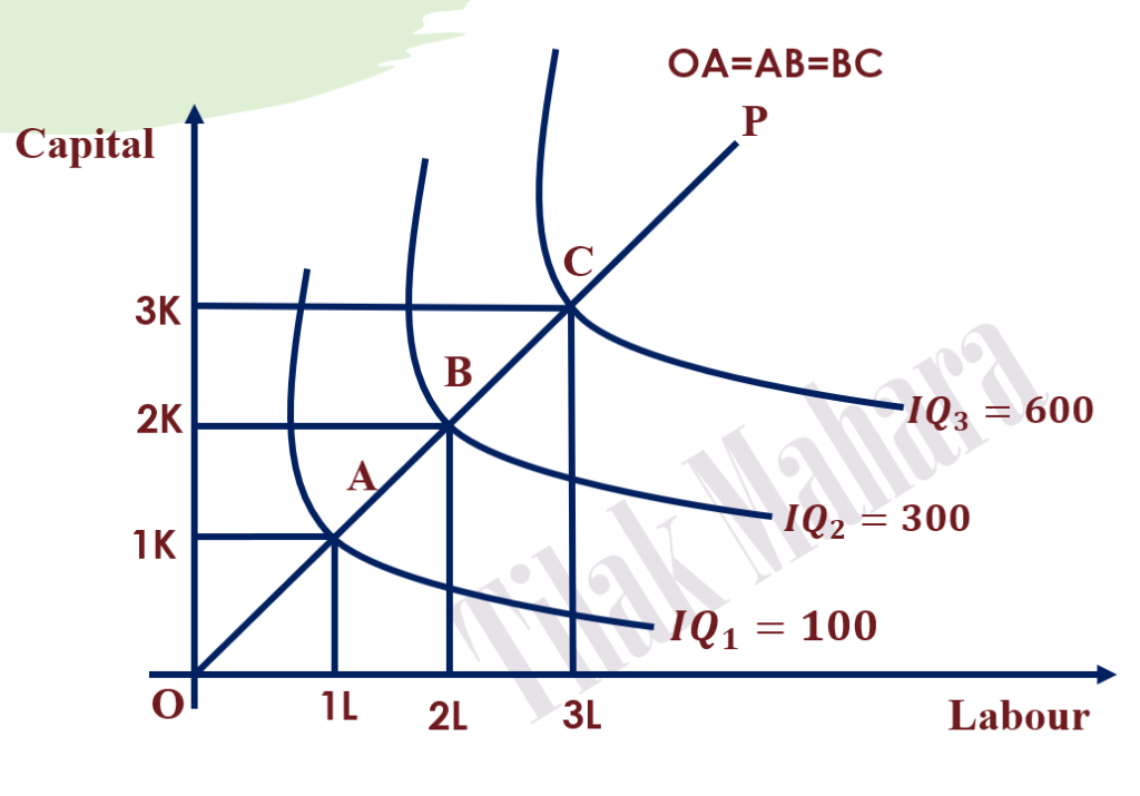
In the above figure, three isoquants IQ1, IQ2, and IQ3 signify output 100 units, 300 units, and 600 units respectively. The distance between these isoquants is equal as OA=AB=BC. This means that there is a constant proportion of the increase in input. But output increase at an increasing rate (i.e. 100 units to 300 units by 200 units and 300 units to 600 units by 300 units). Here, proportionate change in output (ΔQ) is higher than that of inputs (ΔN), so this reflects increasing returns to scale. If we see the product line OP, OA (OK1/OL1) =AB(K1K2/L1L2) = BC(K2K3/L2L3) = 1. This implies that factors or input proportions increase at a constant rate.
Constant Returns to Scale
Constant returns to scale indicate an equal percentage increase in output with the percentage increase in input. It means when the output increases in the same proportion as the increase in all input, it is called constant returns to scale. For example, if all inputs are increased by 10% and output also increases by 10%, it is the case of constant returns to scale. The concept of constant returns to scale can be explained with the help of the following schedule and diagram.
| Combinations | Inputs (In Units) | Output (Units) | Percentage Increase in Input | Percentage Increase in Output |
| A | 1L+1K | 100 | – | – |
| B | 2L+2K | 200 | 100% | 100% |
| C | 3L+3K | 300 | 50% | 50% |
In the above table, combination A exhibits the use of 1 unit of labor and 1 unit of capital and produces 100 units of output. When inputs are doubled or increased by 100 % as shown by movement from combination A to B, output also increases by 100 %. Similarly, movement from combination B to C shows an increase in output by 50 % because of an increase in input by 50%. This shows constant returns to scale.
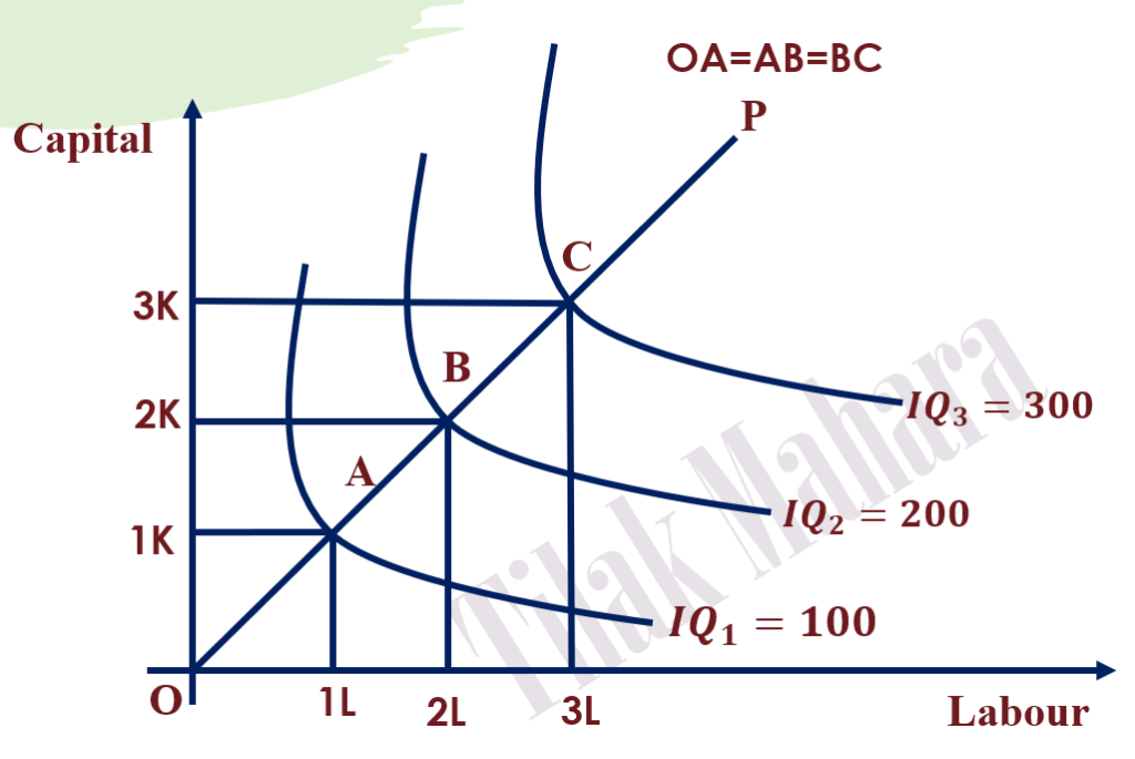
In the above figure, three isoquants IQ1, IQ2, and IQ3 signify output 100 units, 200 units, and 300 units respectively. The distance between these isoquants is equal as OA=AB=BC. This means that there is a constant proportion of the increase in input. Here output also increases at a constant rate (i.e. 100 units to 200 units by 100 units and 200 units to 300 units by 100 units). So, proportionate change in output (ΔQ) is equal to the proportionate change in inputs (ΔN), so this reflects constant returns to scale.
Decreasing Returns to Scale
Decreasing returns to scale indicates a smaller percentage increase in output than the percentage increase in input. It means when the output increases in a lesser proportion than the increase in all input, it is called decreasing returns to scale. For example, if all inputs are increased by 10% and output increases by less than 10%, it is the case of decreasing returns to scale. The concept of decreasing returns to scale can be explained with the help of the following schedule and diagram.
| Combinations | Inputs (In Units) | Output (Units) | Percentage Increase in Input | Percentage Increase in Output |
| A | 1L+1K | 100 | – | – |
| B | 2L+2K | 150 | 100% | 50% |
| C | 3L+3K | 190 | 50% | 26.67% |
In the above table, combination A exhibits the use of 1 unit of labor and 1 unit of capital and produces 100 units of output. When inputs are doubled or increased by 100 % as shown by movement from combination A to B, output increases by 50 %. Similarly, movement from combination B to C shows an increase in output by 26.67 % because of an increase in input by 50%. This shows decreasing returns to scale.
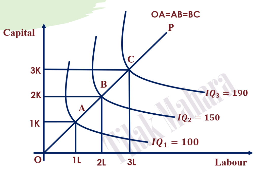
In the above figure, three isoquants IQ1, IQ2, and IQ3 signify output 100 units, 150 units, and 200 units respectively. The distance between these isoquants is equal as OA=AB=BC. This means that there is a constant proportion of the increase in input. But output increase at a decreasing rate (i.e. 100 units to 150 units by 50 units and 150 units to 190 units by 40 units). Here, proportionate change in output (ΔQ) is lower than that of inputs (ΔN), so this reflects decreasing returns to scale.
Alternative Explanation of the Laws of Returns to Scale
Increasing Returns to Scale (IRS)

When increasing returns to scale occur, the successive iso-quants will lie at a decreasingly smaller distance along a product line. As shown in the above figure, the isoquants IQ1, IQ2, and IQ3 represent 100 units, 200 units, and 300 units of output respectively. The distance between the successive iso-quants decreases as OA (OK1/OL1)>AB (K1K2/L1L2)>BC (K2K3/L2L3) representing the smaller increase in inputs labor and capital. But this results in a constant increase in output and shows increasing returns to scale.
Constant Returns to Scale (CRS)
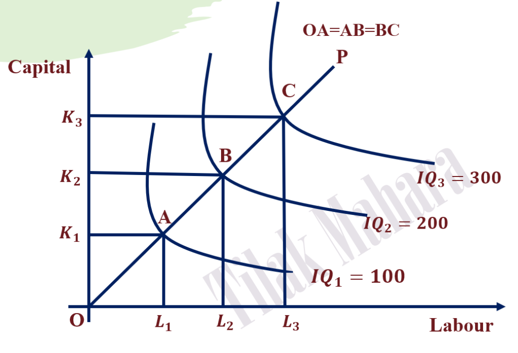
When constant returns to scale occur, the successive iso-quants will lie at the same distance along a product line. As shown in the above figure, the isoquants IQ1, IQ2, and IQ3 represent 100 units, 200 units, and 300 units of output respectively. The distance between the successive iso-quants remains as OA (OK1/OL1) =AB (K1K2/L1L2) =BC (K2K3/L2L3) representing the constant proportionate increase in inputs labor and capital. This results in a constant increase in output too and shows constant returns to scale.
Decreasing Returns to Scale (DRS)

When decreasing returns to scale occur, the successive iso-quants will lie at the increasing distance along a product line. As shown in the above figure, the isoquants IQ1, IQ2, and IQ3 represent 100 units, 200 units, and 300 units of output respectively. The distance between the successive iso-quants increases as OA (OK1/OL1) <AB (K1K2/L1L2) <BC (K2K3/L2L3) representing the expanding proportionate increase in inputs labor and capital. But this results in a constant increase in output and shows decreasing returns to scale.
Causes of the Laws of Returns to Scale
Causes of Increasing Returns to Scale
- Indivisibly of factors of production like machines, management techniques, etc. causes an increase in output with an increase in other individual factor inputs.
- Specialization and division of labor
- External economies expanded by the industry
- Dimensional effects created by internal as well as external economies
Causes of Constant Returns to Scale
- When both economies and diseconomies of scale do not arrive at a certain level of output,
- With indivisible factors when other factors combine optimally
Causes of Decreasing Returns to Scale
- When individual factors become inefficient and less productive
- It becomes difficult to manage the firm efficiently due to difficulties in supervision and coordination of factors
- Inferior factors may be brought into use due to scarcity and exhaustibility of natural resources over time.
- Due to an increase in the prices of factors
- Prices of raw materials go up
- Transport and marketing difficulties may arise in new market areas
- Existence of excess competition among the firms for factors of production and raw materials