Comparative statics tries to establish a relationship between two different interconnected economic variables in two different static situations. Comparative statics is a method of economic analysis that was first used by German economist F. Oppenheimer in 1916.

According to Schumpeter, “Whenever we deal with disturbances of a given state by trying to indicate the static relations obtaining before a given disturbance impinged upon the system and after it had time to work itself out, this method of procedure is known as comparative statics.”

So it is the method of analysis in which different equilibrium situations are compared. 

This analysis compares one equilibrium position with a newly established equilibrium which is formed as a result of a change in the data. It does not analyze the whole path as to how the system grows out from one equilibrium position to another when data have changed. It only explains and compares the initial equilibrium position with the final one reached after the system has adjusted to a change in data.

It can be categorized into two types;

Comparative Micro statics

Comparative Micro statics compares the different equilibrium positions of microeconomic variables at different points in time. We assume that there is no change in the demand and supply functions but due to change in the independent variables the demand or the supply function or both will shift and the market will reach a new equilibrium position generating a new equilibrium price.

This newly generated equilibrium is compared with the old one in comparative micro-statics. Comparative micro statics discusses the process by which the new equilibrium has been arrived at. But it does not provide the answers to the following issues;

• What causes are responsible for breaking the initial equilibrium?
• What is the cause responsible for the establishment of new equilibrium and
• What type of other changes occurred between two equilibriums?

So comparative micro-statics compares the new equilibrium point with the old one but does not study the disequilibrium conditions that emerged between two equilibriums. It can be shown in the following figure:

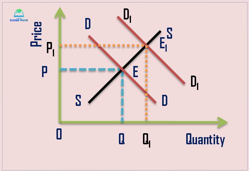
In the above figure, E and E₁ are two equilibrium points. Point E is the original equilibrium when the equilibrium price is OP and equilibrium quantity OQ. Suppose demand increases from D to D₁ due to change in different independent variables (i.e. income, taste, etc.) the new demand curve intersects the supply curve at point E₁ with equilibrium price OP₁ and quantity demanded and supplied OQ₁. The comparative study of two equilibrium points E and E₁ are called comparative micro-statics.

Comparative Macro-statics

Comparative macro-statics tries to establish the relationship between two different interconnected macroeconomic variables in two different macro static positions. It means a comparative study between two different macro static positions is the subject matter of comparative macro statics.

When the initial equilibrium breaks down then the new equilibrium comes up and the comparative macro statics explains how the second equilibrium is different than the first equilibrium. Therefore it is the study of different equilibriums or equilibria at different points in time. Comparative macro-statics compares two still pictures of the economy as a whole. It can be shown in the following diagram;

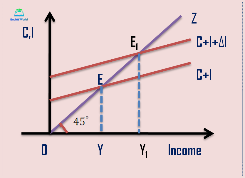
In the above Keynesian income determination model, the initial equilibrium existed at point E-the intersection point between the aggregate demand function and aggregate supply function of the economy. When the aggregative demand function shifts upward from C+I to C+I+ delta I due to an increase in investment the new equilibrium point of the economy is obtained at point E₁.

With the change in equilibrium from point E to E₁, the national income also increased from Y to Y1. In such a way the economy has moved from one still picture to another still picture represented by a movement from point E to E1. Comparative macro-statics is concerned with the comparative study of these two static points of an entire economy rather than studying the disequilibrium phases that take place between them.

Importance

In the real world, a complete and true analysis of the changing phenomenon of daily life would be the dynamic analysis. However comparative statics is a very useful technique for explaining the changing phenomenon and its crucial aspects without complicating the analysis.

According to Hicks, this method is praiseworthy for analyzing the effects of causes that bring about disturbances. It re-establishes stability in the process of change. If there are some changes in economic variables that lead to the process of continuing changes, it is not possible to tell when this process will end.

Similarly, if once there is a disturbance in the equilibrium which begins a continuous process of instability, it is not possible to tell definitely when the equilibrium situation will be restored.   In such a situation, comparative statics can show the direction of change by pointing towards some definite point of equilibrium. Thus this analysis provides certainty in an uncertain situation.  

Limitations

It has the following limitations

• It has limited scope as it excludes many important economic problems. The problems relating to economic fluctuations and growth are not included in comparative statics.
• It is unable to explain the process of change from one position of equilibrium to a new equilibrium position. It shows only a partial picture of the economic relationship.
• This method is unable to say the time period of the adjustment process. It means comparative statics is not sure when the new equilibrium will be established as it neglects the disequilibrium adjustments and their time coverage.

Conclusion

Comparative static analysis always compares one equilibrium positive with another when the data related to variables undertaken in the model are changed and finally reached another equilibrium position. Thus, in this analysis, two different static equilibriums representing two different times are compared. It does not study the time taken by the system to reach the new equilibrium level after breaking down the initial one. It also ignores all the ups and downs between old and new equilibrium.

References

Ahuja, H.L. (2017). Advanced Economic Theory. New Delhi: S. Chand and Company.

Jhingan, M.L (2012). Advanced Economic Theory. New Delhi: Vrinda Publications (P) LTD.

Maddala, G.S., & Miller, Ellen. (2004). Microeconomics Theory and Applications. Chennai: McGraw Hill Education (India) Private Limited.