Dynamics is the part of economic analysis that deals with whether an economic system in disequilibrium reaches an equilibrium position, how long it takes, and the path it follows to do such. Dynamic refers to the evolutionary process in a dynamic manner. This method of economic analysis takes into account all the changes, lags, sequences, cumulative magnitudes, and expectations also.

It picturized the entire series of adjustments that take place between the break-up of old equilibrium and the formation of a new one. Dynamics represent a continuing picture of the working of the national economy. Thus, it is a realistic method of study and investigation of the relationships between economic variables. It is the most comprehensive and at the same time complex method of analysis in economics. 

According to Prof. Ackley, “Dynamics is concerned essentially with states of disequilibrium and with change.”

J.A. Schumpeter defines economic dynamics as, “We call a relationship dynamic if it connects economic quantities that refer to different points of time. Thus, if the quantity of a commodity that is offered at a point of time (t) is considered as dependent upon the price that prevailed at the point of time (t-1), this is a dynamic relation.”

According to Ragnar Frisch who is one of the pioneers in the use of dynamic techniques in economics, “A system is dynamical if its behavior over time is determined by functional equations in which variables at different points of time are involved in an essential way.” 

It is thus the analysis of the process of change that continues over time. Economy over time may take place change in two ways. The first one is without changing its pattern and the second one is by changing its pattern. Economic dynamics are related to the second type of change.

For example, if there is a change in the population, capital, production techniques, and business forms in any one or all of them the economy will assume to follow a different pattern and will change its direction.

In economics, many micro and macroeconomic relationships can be presented as an example of economic dynamics. If the supply (S) for a good in the market in the given time (t) depends upon the price that prevails in the preceding period (t-1), the relationship between supply and price is said to be dynamic.

So the dynamic relationship can be expressed as; S_t=f (P_t-1)

Where S_t is the supply of goods in a given time ‘t’ and P_t-1 is the price in the preceding period.

Similarly, the demand (D) for a good in the market in the given time (t) depends upon the price that prevails in the preceding period (t-1), the relationship between demand and price is said to be dynamic.

D_t=f (P_t+1)

Where D_t indicates quantity demanded in a time ‘t’ and P_t+1 is the expected price in the succeeding period. So if one considers quantity demand (D) at a time period t as a function of the expected price in the succeeding period (t+1), the relation between demand and price will be called dynamic and the analysis of such relationships would be called economic dynamics.

In macroeconomics, the example of economic dynamics can be given with the help of the consumption function. If the consumption of an economy in a given time depends upon the income in the preceding period (t-1), it is called dynamic relation.

This can be expressed as follows; C_t=f (Y_t-1)

The dynamic analysis can be explained in terms of micro and macro dynamic models.

Micro Dynamics/Cobweb Model

Microdynamics explains the lagged relationship between the microeconomic variables. It deals with the procedure by which the new equilibrium in the market is formed. Microdynamics explains all types of changes that occurred between two equilibrium points.

It can find the path followed by the system over time in moving from the old to the new equilibrium. Microdynamics also analyzes the time taken by the system to reach a new point of equilibrium after getting disturbed from its initial equilibrium.

The Cobweb model is used to analyze the dynamic relationship between market demand, market supply, and price.  The Cobweb model or Cobweb theory was developed by Nicholas Kaldor in 1934. The cobweb model is an economic model that tells why prices might be subject to episodic or periodic fluctuations in a certain type of market.

It casually describes the supply and demand in a market. This model is more applied in the agricultural market. There are many perishable agricultural commodities whose price and outputs are determined over long periods and they show cyclical movements. With cyclical fluctuations in prices quantities produced also see, to move up and down in counter-cyclic manners. Such cyclic functions are explained with the help of the Cobweb model. It means the Cobweb theory is applied to explain the dynamics of demand, supply, and price over long periods.

Let us assume that the production process spreads over two periods as current (t) and previous (t-1). The production in time ‘t’ is assumed to be determined by decisions made in the period ‘t-1’.  Thus the current output reflects a production decision made by the producer during the previous period.

This decision is in response to the price that the producer expects to rule during the current period when the crop is available for sale.  But the producer expects that price that would be existed throughout the current period would equal the price during the previous period. (i.e. P_t=P_t-1).

Assumptions

The Cobweb model is based on the following assumptions;

• The current year’s (t) supply depends upon the last year’s (previous year’s) (t-1) decisions regarding output level. Thus, the current output is influenced by last year’s price.
• The current year is divided into sub-periods of a week or fortnight.
• The parameters determining the supply functions have constant values over a series of periods.
•  Current demand (D_t) for the product is a function of the current price (P_t)
• The price expected to prevail in the current period is equal to last year’s price.
• The commodity under consideration is perishable and can be stored only for one year.
• Demand and supply both are linear functions.

The model

There are three forms of the Cobweb model; Convergent Cobweb, Divergent Cobweb, and Continues Cobweb model.

Convergent Cobweb

The demand function D_t=f (P_t+1) and supply function S_t=f (P_t-1). The equilibrium will be when the quantity supplied equals the quantity demanded. Thus D_t= S_t.

The equilibrium in the market system where the producer’s current supply is determined based on the price of last year or the previous year can be established only through a series of adjustments that take place over several consecutive periods. This concept is explained with the help of the following figure;

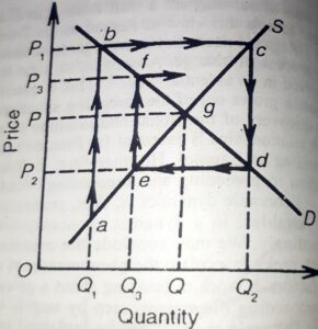
Assume the producer is producing one particular crop for a year. The amount of production (supply) is decided on the assumption that the price for that product in the current year will be exactly equal to the price of last year. The market demand and supply curve of the market are denoted by D and S respectively.

Last Year

• Last year these two curves intersected with each other at point E-equilibrium point with equilibrium price OP and OQ equilibrium quantity of demand and supply. So last year’s price and quantity are OP and OQ.

Let us consider that something has happened (like shock in the external environment as COVID-19) and as a result market is disturbed and the current output is decreased to OQ₁ less than the output of last year.

Period-1

• Due to external disturbance in the system, supply decreased to OQ1 less than the equilibrium output of last year
• This leads to a rise in the price of OP1 in the current year.
• The story ended here for the first year.

Period-2

• For period 2 the suppliers decide to supply based on the previous period’s price because they assume this year’s price (price in period 2) is equal to the price that existed in period 1.

• So producers expect that this price (OP₁) prevails in the market for at least one year and as a result, they increase their production and supply OQ₂ quantity in the market.
• So supply in period 2 is the function of the piece in period 1.
• But this is also the case of disequilibrium. This supply is higher than the quantity needed in the market. Here quantity needed in the market is OQ but supplied is OQ₂.
• This will reduce the price up to OP₂.
• The story of period 2 ends here.

Period-3

• In period 3 the quantity supply is a function of price in period 2. So the quantity supply in period 3 is smaller than the quantity demanded in the market.
• The quantity supply is OQ₃ as a function of price OP₂.
• Here supplied quantity OQ₃ is less than the quantity demanded in the market.
• This will again increase the market price and will become more than OP. this is the end of the story in period 3.

Period-4

• In period 4 the quantity supply will base on the price of period 3.
• This means quantity supply in period 4 will increase and become more than demanded (more than OQ)
• This will reduce the price and it will become less than OP. This is the end of the story in period 4.

Period-5 and 6

• The supply in period 5 is the function of the reduced price of period 4.
• So quantity supply is also reduced and remains below the demanded quantity.
• This will again increase the price in the market.
• With an increase in price in period 5 the supply in period 6 is increased. 

If this process goes continuously following the same manner the system ultimately reached the interaction point of demand and supply D and S respectively. This is point ‘g’ in the out diagram.  So the sequence of adjustment describes the pattern as Cobweb from point ‘a’ to ‘g’.

The disequilibrium emerged at point ‘a’ is finally reached point ‘g’ with continuous changes in price and quantities. This is called convergent and dynamic equilibrium with lagged adjustment. The equilibrium will be convergent when the slope of the demand curve is lower than the slope of the supply curve. It is the case of the steeper supply curve and flatter demand curve or supply curve is less elastic than the demand curve then it is the case of convergent disturbance. 

Divergent Cobweb

If instability in equilibrium does not convert into original equilibrium and price and quantities move away from the initial position then it is called divergent. It is explained in the following diagram;

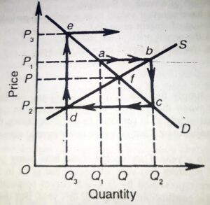
The initial equilibrium price is OP and the equilibrium quantity is OQ. Suppose there is an emergence of disturbance and as a result quantity supplied decreased to OQ₁.

Period-1

As a result of external shock, there is a decrease in quantity supply to OQ₁ and so the price is increased to OP₁.  

Period-2

The quantity supplied in period 2 is the function of the price in period 1. So there is an increase in quantity supply in period 2 and becomes OQ2. It is more than the equilibrium quantity OQ. As a result, the price decreased in this period to OP₂.

Period -3

Supply in period 3 is a function of price OP₂. Since there is a direct relationship between price and supply quantity so supply in period 3 is OQ₁. There is a greater shortage in the market. And the price is increased. In this period price becomes OP₃.

Period-4 and next to all

The supply quantity in period 4 is the function of price in period 3. It will increase the quantity of supply more and reduces the price. The price in such a period will become less than OP₂. This will further reduce the quantity supply in period 5. Price in the next period will become higher.

In such a way price-quaintly leads the system far away from the original equilibrium. This shows an explosive situation and unstable equilibrium. It is the case of divergent Cobweb. When the slope of the demand curve is greater than the slope of the supply curve, the price will diverge from the equilibrium. In this case, the supply curve is flatter and the demand curve is steeper.

Continues Cobweb

When the slope of the supply and demand curve is the same then the equilibrium price will oscillate around its equilibrium value by making a circle. It means the elasticity of supply is equal to the elasticity of demand. It can be explained with the help of the following diagram;

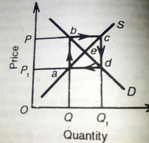
In the above figure, D is the demand and S is the supply.

Period-1

Suppose there is an OQ₁ quantity of supply in the first period. This is a higher quantity. So it will reduce the price up to P₁.

Period-2

In period 2 the quantity supply is determined by the price measured in period 1. So quantity supply is OQ in period 2. This is lower than the OQ1. A lower quantity will increase the price and becomes OP.

Period-3

In period 3, the quantity supply is the function of price in period 2. OP was the price in period 2 which was higher. So this will lead to a higher supply in period 3 which is OQ₁ equivalent to period 1. This will lower the price again to OP₁.

Period-4

In period 4 quantity supply is OQ as s function of price OP₁. This supply is equivalent to the supply of period 2.

In such a way all the subsequent periods will move towards OP, OP₁, OQ, and OQ₁. Here the price is entirely measured by the current supply and supply is completely based on the price of the previous period. So functions in price and supply or production in such a situation are continuously moved in this particular cyclical pattern infinitely and will not make or form any equilibrium. This case is true when it is exact but the opposite slope of demand and supply. These are also called continuous fluctuations.  

Macro-Dynamics

When macroeconomic relationships are treated dynamically then such analysis is known as macro-dynamics. Samuelson, Kalecki, and Post-Keynesian like Harrods, and Hicks have greatly dynamited the macroeconomic theories of Keynes.

So macro-dynamics refer to a position by which the system passes from one position of equilibrium to another. It analyzes the path taken by the macro variables to move from the old equilibrium to the new equilibrium. It also takes into consideration the time taken by the system to reach a new equilibrium position after getting disturbed from its initial equilibrium position.

Thus, macro-dynamics studies the transformation from one position to another through a continuous series of disequilibrium. It is as a rule inclusive and complete process of economic analysis. It presents a full account of all the development taking place in the economy in the transitional period between the break-up of the old equilibrium and the establishment of the new.   

According to Kurihara, “Macro-dynamics treats discrete movements or rates of change of macro variables. This method separates the process of trial and error into a series of continuously changing reactions and indicates step by step what the cause is and what the effect is. It describes the changing universe as it is related to previous or subsequent adjustments, it analysis the discrete and continuous changes of aggregate, the sequence of cause-and-effect events arising from some initial disturbance, and the time-paths of macro-variables and aggregative relationships. Thus, the macro-dynamic method enables one to see a motion-picture of the functioning of the economy as a progressive whole.”

The macro-dynamic model can be explained with help of the Keynesian process of income propagation where consumption is a function of income of the preceding period (C_t=f {Y_t-1} and investment is a function of constant autonomous investment I= f {( DI}.

This is further explained with the help of the following diagram;

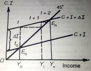
In the above figure, C+I is the aggregate demand function and the 45 line is the aggregate supply function. In the time t0 the economy is at equilibrium at point E₀ with the equilibrium level of national income ‘Yo‘. Suppose there is a change in investment represented by ‘I’ then in period t₁ income increased from Y₀ to Y₁. It is represented by a higher aggregate demand curve C+I+DI.

But in period ‘t’, consumption lags and is still equal to the income at E₀. In period ‘t+1‘ consumption rises and along with the new investment there is an increase in income (beyond OY₁). This procedure of income flow will go on till the aggregate demand function C+I+ DI intersect the aggregate supply function line at E_n in the n^th period and the new equilibrium income level is determined at OY_n. The curves steps t₀ to E_n show the macro-dynamic path. Thus there is a movement in the equilibrium position from point E₀ to E₁. Macro dynamics deals with the path taken by the economy to move from E₀ to E_1.

Need and Significance of Economic Dynamics

The use of economic dynamics is essential if one wants to make a realistic analysis of economic relationships. In practical life, almost all the economic variables like price, income, investment, saving, and consumption are always changing. So the account of these all changes and their effect on an economic relationship is explained by economic dynamics.

The major significance of economic dynamics are pointed as below;

• It is realistic and not imaginary and explains the causes and effect relationship of changing economic phenomena and enables us to see a moving picture of the working of an economy.
• It studies the entire process of stability of equilibrium. The behavior of the economic system is reflected by different ups and downs of economic relations.
• The problems including time lags, rates of growth, and sequence analysis require the compulsorily use of macro dynamics. Certain economic circumstances and their effect on development are studied in dynamics.
• It is essential in the study of the business cycle.
• The techniques of economic dynamics are essential in the development of new techniques of economic analysis. An econometric model of national income, trade cycle, and economic growth are built-in economic dynamics.

Limitations

It has the following limitations

• Economic dynamics is a complex and intricate method of economic analysis.
• It may lack favorable conditions in the study of fundamental human behavior. Human wants may not obey the theoretical assumptions of the model. Some empirical findings under economic dynamics may lack theoretical foundations.
• It has made economics difficult, and complex for ordinary learners of economics. So it has itself created practical applicability of dynamics.

Conclusion

Economic dynamics is very popular in recent economic analyses. It is a more realistic method of analyzing the behavior of economic units and the economy as a whole. In economic dynamics, there is a due reorganization of time elements of the given variables to each other in the relationship.

All types of interactions between the variable in the model are studied in detail. Dynamics explains the lagged relationship between economic variables. It throws full light on what is happening in the system during the period of transition from initial static equilibrium to another or final. It is a detailed study of disequilibrium.   

References

Ahuja, H.L. (2017). Advanced Economic Theory. New Delhi: S. Chand and Company.

Jhingan, M.L (2012). Advanced Economic Theory. New Delhi: Vrinda Publications (P) LTD.

Maddala, G.S., & Miller, Ellen. (2004). Microeconomics Theory and Applications. Chennai: McGraw Hill Education (India) Private Limited.