Introduction to Consumer’s Equilibrium

The prime objective of a consumer of goods and services is to derive the maximum or optimum level of satisfaction or pleasure or happiness keeping himself or herself within a fixed amount of budget or money income. Here we will discuss consumer’s equilibrium through the indifference curve approach. A consumer is said to be in equilibrium with the combination of two goods purchased that maximizes total utility, given his/her income and the price of the two commodities.

We combine the indifference curves and the budget line on the same diagram to illustrate the consumer’s equilibrium. The indifference curve shows the consumer’s preference, it tells about what the consumer is willing to buy. The budget line displays the consumer’s ability to pay. When we see the situation in which the indifference curve and the budget line come together, we can find the amounts of every good that the buyer is willing well as able to buy. Therefore, a consumer targeting to optimize the utility or satisfaction will have to choose a blend of two commodities available on his/her price line and acceptable by the possible upper achievable indifference curve.  If the consumer is in the possible highest-reach indifference curve and has allowed his/her budget limit, then we can say that the consumer is in equilibrium.   

Consumer equilibrium is, therefore, a situation in which the consumer with his limited income maximizes his level of satisfaction in the process of consuming goods. Thus, it is the point at which the consumer attains maximum satisfaction. Speaking in mathematical language, satisfaction maximizes at the point where an indifference curve is tangent to the budget line. At the equilibrium point, the slope of the indifference curve (measures the consumer’s marginal rate of substitution) is equal to the slope of the budget line (signifies the opportunity cost of one commodity in relation to the other measured by market prices). After the realization of such a situation, the buyer does not want to move towards another combination until the prices and income of the consumer remain the same.

Assumptions of Consumer’s Equilibrium

The consumer’s equilibrium under the indifference curve approach is based on the following assumptions.

Conditions Needed for Consumer’s Equilibrium

Based on the above-mentioned assumptions, the consumer’s equilibrium point can be defined with the help of the following conditions. It means. The indifference curve approach requires the following two conditions to make sure about the equilibrium point of a consumer (consumer’s equilibrium).

Necessary Condition/the First Order Condition

The first-order condition or the necessary condition for the consumer’s equilibrium is that the budget line should be tangent to the Indifference curve. i.e. the slope of the budget line is exactly equal to the slope of the indifference curve is the necessary condition for the consumer to attain equilibrium under the ordinal approach. In the technical language, the first-order condition requires equality between the marginal rate of substitution and the ratio of commodity prices.

Thus, the necessary condition is;

The slope of IC= Slope of PL

Supplementary or Second-Order or Sufficient Condition

The first-order condition or the necessary condition may not always be able to fix identify the consumer’s equilibrium point.  Thus, the consumer’s equilibrium under the indifference curve approach requires sufficient conditions as well. The convexity of the indifference curve towards the origin is sufficient condition i.e., MRS_{X, Y} is diminishing. It means MRS_{X, Y} must be diminishing at the point of the consumer’s equilibrium. This condition will allow the buyer to conquer a stable equilibrium.

Graphical Presentation of Consumer’s Equilibrium

The following figure displays the graphical presentation of the consumer’s equilibrium condition.

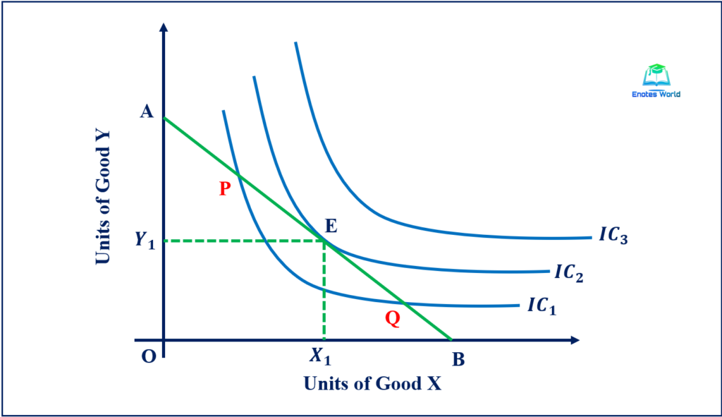
In the figure above, there are three indifference curves, IC1, IC2, and IC3 presenting a hypothetical indifference map of the consumer. AB is the hypothetical budget line. We see that the budget line AB is tangent to the indifference curve IC2. It means at point E; the slope of the indifference curve and the slope of the price line are equal to each other. So, the consumer attains maximum satisfaction at the given level of income at point E.  

The budget line AB intersects IC₁ at points P and Q which suggests the possibility that IC1 can achieve by using the same budget line. But IC1 gives lower satisfaction than IC2. Thus, a rational consumer rejects to choose IC1. IC3 gives higher satisfaction than IC2 but it cannot be attained under the given budget constraints presented by line AB. So, point E is the consumer’s equilibrium position. at point E slope of IC and the slope of the budget, line are equal as {MU_X/MU_Y=P_X/P_Y}  

The sufficient condition for the consumer’s equilibrium requires that the IC must be convex to the origin at the point of tangency so that the law of diminishing marginal rate of substitution is secure. The meeting of necessary conditions (MRS between two goods equal to the price ratios) only does not guarantee whether the satisfaction attained by the buyers is maximum or not. Thus, the following figure shows the attainment of the consumer’s equilibrium with the fulfillment of both necessary and sufficient conditions.

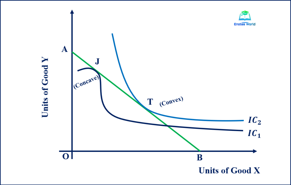
In the figure, there are two tangency points J and T on IC₁ and IC₂ respectively with the same budget line AB. So here the first-order condition has been fulfilled at both of the points. However, point T lies on the higher indifference curve (IC2) and J lies on the lower indifference curve (IC1). Here, IC1 ensures a lower level of pleasure and IC₂ ensures a higher level of pleasure. Similarly, at point J the indifference curve IC₁ is concave to the origin. At point T, the IC₂ is convex to the origin with a higher level of satisfaction.

Thus, we can say that at the point of tangency of the budget line and IC, the indifference curve must be convex to the origin for the maximization of satisfaction as a higher attainable indifference curve gives a higher level of pleasure and consumers always prefer more to less of goods.  Point T of the above figure has fulfilled both of the conditions for the attainment of the consumer’s equilibrium.

Mathematical Conditions for Consumer’s Equilibrium

In the mathematical language, the following expressions show the necessary and sufficient conditions for consumers’ equilibrium.

Necessary Condition

At the point of tangency, the slope of IC=slope of the price line

Where the slope of IC= ∆Y / ∆X=MRS _{X, Y} =-MU_X/MU_Y; the slope of the budget line =-P_X/P_Y

Thus, we have -P_X/P_Y=-MU_X/MU_Y

So, the first-order condition is P_X/P_Y=MU_X/MU_Y

Sufficient Condition

The second-order condition or the sufficient condition requires the convexity of the indifference curve at the point of tangency between the price line and the indifference curve. It means, at the point of tangency the rate of change in the slope of IC should be positive. That is the second-order derivative of the utility function must be positive. Mathematically,

∆²Y/∆X²=d²Y/dX²>0

Therefore, the consumer’s equilibrium under ordinal utility analysis is achieved at the point of tangency between the indifference curve and price line and the convexity of IC at the point of tangency.  

References and Suggesting Readings

Ahuja, H.L. (2017). Advance Economic Theory. New Delhi: S. Chand & Company.   

Dwivedi, D. N. (2018). Microeconomics Theory and Application. New Delhi: Vikas Publishing House PVT LTD

Kanel, N.R. and et. al. (2019). Microeconomics for Business. Kathmandu: Buddha Publications.