Meaning of Stable Equilibrium

If any small disturbances take place forces come into play to re-establishes in the initial position is called stable equilibrium. It means after any fluctuations either in the price or quantity supplied or demanded if these market forces again come back or move back to the original equilibrium position then such equilibrium is called stable equilibrium. So in the case of stable equilibrium, there is a tendency for the disturbed or affected market forces to return or move back to the original equilibrium.

The existence of equilibrium does not ensure that such equilibrium is or is not a stable one. So stability test is the next distinct issue or problem connected with the equilibrium.

The case of stable and unstable equilibrium can be shown with the help of the following diagrams.

In figure-1 point, e shows the equilibrium point in the market with corresponding equilibrium market price OP and quantity demanded and supplied OQ. Let us consider that the disturbing price is OP1 (higher than the equilibrium price). At OP1 price there is excess supply in the market represented by portion ab. Excess supply pushes the price down due to the competition between sellers and the price will fall continuously until it reaches the original equilibrium position OP.

If we consider OP₂ (below equilibrium price) the disturbing price then we can see that at OP₂ there is excess demand represented by ‘fg’. Excess demand pulls prices up due to the competition between the buyers. This process goes on continually until the price again reaches the original equilibrium price OP.

So the disturbing price is moved again towards the original equilibrium price and accordingly, quantity demanded and supplied also. Thus this has shown that equilibrium is a stable equilibrium.

In the figure-2 also point, e shows the equilibrium in the market. Suppose OP₁ is a disturbing price and at such price, there is excess demand represented by ‘ij’. There is positive excess demand and supply is very low so the price is to be further increased to reduce the demand. With a further increase in price, it goes far away from the original equilibrium and never comes back.

If the disturbing price is OP₂ then at such price there is excess supply represented by ‘kl‘. Since there are excess supply and less demand in the market the price is to be further reduced to encourage demand and discourage further supply. With a reduction in price, it goes far away from the original equilibrium price and never comes back to the original position.

Thus, the case shown in figure-2 is the case of unstable equilibrium. It is due to the unusual behavior of the demand and supply curve. Upward sloping demand and downward sloping supply curve never generate stable equilibrium.

Excess Demand Function Approach to Stability of Equilibrium

It is an alternative approach to seeing the stability of equilibrium. In the excess demand functions approach, we see the slope of the excess demand function at the intersection point to the price axis. Since excess demand is the function of price so it should be negatively sloped at the intersection point of the excess demand curve and price axis. And at that point, it should have zero excess demand also. It can be explained with the help of the following diagrams;

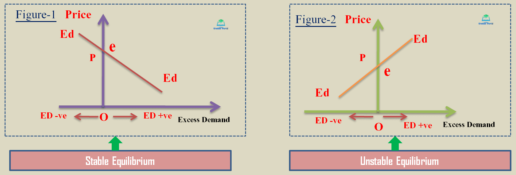
In figure-1 the excess demand curve has intersected the price axis at point e-equilibrium point with a positive price. At point e there is zero excess demand and the slope of the excess demand curve is also negative.

This ensures that equilibrium is stable. At the equilibrium point, the equilibrium price OP is determined. At any price beyond OP, there is negative excess demand. Negative excess demand indicates a higher supply than the quantity demanded in the market. This will create competition between sellers and finally bid down the price and ultimately the price will become OP.

Similarly, if the price is below OP, there is positive excess demand. It means demand is higher than the quantity supplied in the market. This will bid up the price until it will again become OP. Thus, figure-1 shows a stable equilibrium.

In the figure-2 also the excess demand curve intersects the price axis at point e-equilibrium point with zero excess demand and positive price OP. But the slope of the excess demand function at the point of intersection is upward sloping which is the unusual behavior of the excess demand function. This will generate an unstable equilibrium.

Any price above OP, there is positive excess demand and which will further increase the price and it never comes back to the original price OP. Similarly, at any price below OP, there is negative excess demand and it will further decrease the price in such a way that it will never come back to its original position OP. Thus in this case the generated equilibrium is an unstable one.

Conclusion

The stability of equilibrium thus requires a single equilibrium price with a corresponding quantity of demand and supply. The equilibrium is called stable when it’s pulling and pushing forces to bring it back to the original equilibrium position after fluctuations and disturbances in its operation and its variables. A balanced state is ultimately restored in case of stability. The opposite of it is called unstable equilibrium. Unstable equilibrium never comes back and never restores to the original state of balance.

Reference

Koutsoyiannis, A.(1979). Modern Microeconomics. London: ELBS/Macmillan