The uniqueness of equilibrium is referred to the query of the number of times that equilibrium exists and corresponded values are determined in the particular model or system. If there is a single equilibrium that is the demand curve and supply curve meets only one time at a single positive price with the corresponding positive quantity of supply and demand then this is called a unique equilibrium.  

Thus uniqueness of equilibrium implies that there exists only one positive price and at such price demand equals supply or there is zero excess demand at such price. So if there are two or more prices with corresponding quantities then it is the case of multiple equilibria and in the case of multiple equilibria, the uniqueness of equilibrium is not found. In the case of the labor market, there may be multiple equilibria and such equilibriums are not unique equilibriums.  

We might have some cases in which demand or supply or both of the forces may not behave normally and as a result, there exist two or more positive prices and corresponding demand and supply quantities. The uniqueness of the equilibrium can be further explained with the help of the following diagrams;

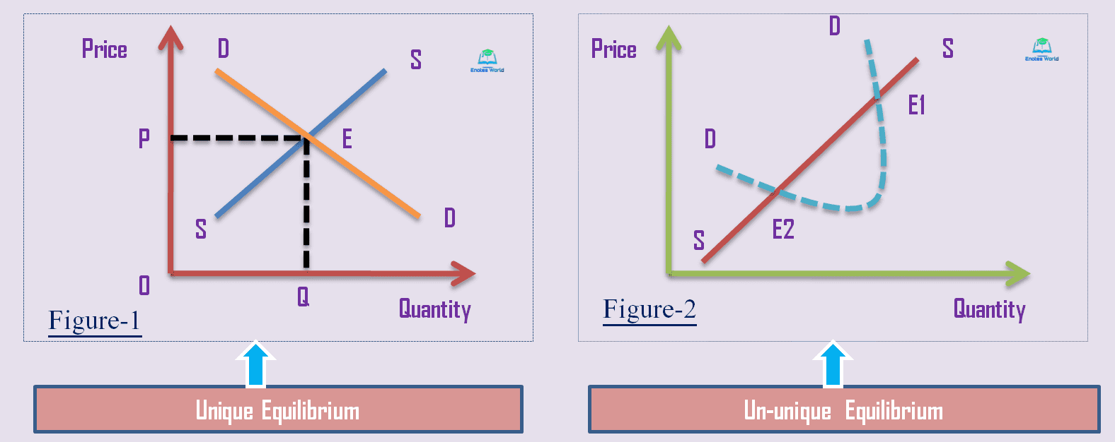
In figure-1 downward sloping demand curve and upward sloping supply curve intersected with each other at point E-equilibrium with equilibrium price OP and equilibrium quantity of demand and supply OQ. There is only one positive price and corresponding quantities (demand and supply intersected only one time) therefore the equilibrium shown in figure-1 is called a unique equilibrium.

Similarly, in figure-2 the demand curve intersects the supply curve at points E₁ and E₂. These two points are equilibrium points formed by given demand and supply curves. It is the case of multiple equilibria. They meet more than one time and thus there are two equilibriums. This figure thus does not show the unique equilibrium. It means neither of the equilibrium is a unique one.

Excess Demand Function Approach to Uniqueness of Equilibrium

We know that under the excess demand function approach the equilibrium exists when the excess demand function cuts the price axis at a positive price and at that point there is zero excess demand. For stability, the slope of the excess demand curve should be negative.

While looking for the uniqueness of the equilibrium we have to look at how many times the downward sloping excess demand function or curve has intersected the price axis. If it cuts only one time then the equilibrium is considered unique and vice versa. This can be further explained with the help of the following diagram;

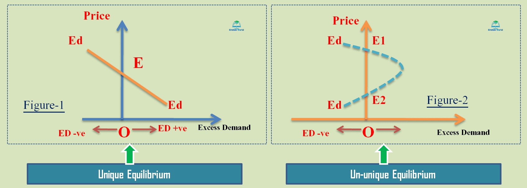
The above diagram shows the testing of the uniqueness issue of the equilibrium under the excess demand function approach. In the figure-1 the downward sloping excess demand function intersects the vertical price axis only one time at point E-equilibrium point. At point E there is zero excess demand. Thus the equilibrium depicts in the figure-1 is a unique equilibrium.

Similarly, in figure-2 the excess demand function or curve intersects the vertical price axis and generated equilibrium. But in this case, the excess demand function has cut the price line two times and generated multiple equilibriums. The multiple equilibrium case is known as equilibria. In the case of multiple equilibria or if the excess demand curve cuts the price line more than one time then neither of the equilibrium is considered a unique equilibrium. So the equilibrium points E₁ and E₂ both are un-unique equilibrium.

Summary

Thus uniqueness of the equilibrium deals with whether or not there exists only one positive price and at such price demand equals supply or there is zero excess demand at such price. Equilibrium is called unique if there is only one or a single equilibrium point. If the opposite market forces interact two or more times in a single model then the uniqueness of the equilibrium is destroyed. It is a rare case in the real world. However, in the case of the backward bending labor supply curve, we can see the multiple equilibriums in the model.  

References

Koutsoyiannis, A.(1979). Modern Microeconomics. London: ELBS/Macmillan